Pore Pressure Estimation – What Can We Learn From 4D?

Summary

Most methods for pressure prediction from seismic are based on detection of low velocity anomalies. The significant growth of time-lapse seismic surveys gives us a possibility to check the robustness and limitations of these classical prediction methods, and might also lead to new methods for pressure prediction that can be used in exploration. Using a simple geo-mechanical model (Hertz-Mindlin) it is shown that the AVO-response of a pressure anomaly is opposite of for instance a fluid anomaly. It is suggested that these simple AVO-observations could be combined with more conventional methods, in order to reduce the uncertainty in pressure prediction from seismic. Main limitations are the validity of the geo-mechanical model, the assumption of constant lithology between the normal and anomalous segments and the validity of the Gassmann model. A 4Dexample from a 30% porosity sandstone reservoir shows that a 5- 7 MPa pore pressure increase leads to an amplitude change at the top reservoir interface that is explained by approximately 20% decrease in P-wave velocity.

The observed pull-down effect (time lapse travel-time shift) measured over the whole reservoir thickness is of the order of only 4-6 ms, indicating a gradual change in velocity below the top reservoir event, decreasing with depth. Time-lapse velocity analysis is not precise enough to pick up this gradual velocity change between the two surveys. 4D data from segments undergoing a pore pressure decrease of 2-4 MPa does not show amplitude or travel-time shifts above the background noise level. Thus one might say that 4D observations indicate that over-pressured rocks should be easier to detect by seismic methods than rocks with anomalous low pore pressure.

Introduction

Interpretation of time-lapse seismic data depends on knowledge of the relation between the seismic parameters and typical reservoir parameters we want to map, as for instance pore pressure changes and fluid saturation changes. The established link for bridging the gap between the two types of parameters is rock physics. For saturation effects, the Gassmann equations form a reasonable working platform, enabling us to make quantitative estimates for how much each of the seismic parameters changes with for instance water saturation. However, for pore pressure changes, I claim that the corresponding platform is weaker: we have to rely on ultrasonic core measurements in order to establish a link between pore pressure changes and corresponding changes in seismic parameters. One major weakness of the core measurements is that the core sample is damaged during the coring process (Nes et al., 2000). Artificial cracks are probably formed during the anisotropic stress unloading process. Even if the core sample is reloaded to simulate in situ stress conditions for the ultrasonic core measurements, it is not very likely to assume that the original crack state of the sample is re-established again. Furthermore, we have to deal with the upscaling problem for our core measurements: Is the ultrasonic measurements made at the small core sample representative at seismic scale?

The Hertz-Mindlin model: an attempt to relate velocity to pressure

Various contact models have been proposed to estimate effective moduli of a rock. Some of these models are presented by Mavko, Mukerji and Dvorkin in their rock physics handbook, 1998. The Hertz-Mindlin model (Mindlin, 1949) can be used to describe the properties of precompacted granular rocks. The effective bulk modulus of a dry random identical sphere packing is given by

and the effective shear modulus is given by

where ν and μ are the Poisson’s ratio and shear modulus of the solid grains, respectively, φ is the porosity, C is the average number of contacts per grain and is the effective or net pressure.

The relation between net stress and reservoir pore pressure can be defined as (see for instance Christensen and Wang, 1985):

where P is effective pressure, Pext is external pressure, P_porc is pore pressure, and η is the coefficient of internal deformation, a usually unknown parameter, often assumed to be close to one. However, if differs from one, this will lead to stretching of the velocity versus pressure curves, and hence a corresponding increase in the uncertainty associated with the estimated pressure and saturation changes. The fact that we actually do not know the internal deformation coefficient η, is a limiting factor for quantitative use of rock physics measurements for pore pressure estimation. In a rock physics experiment, we measure the net or effective pressure (P), while in a reservoir, we measure the pore pressure (P_pore).

The P(V_p) and S(V_s) wave velocities are now given as

The density is

where ρ_f and ρ_ma are the fluid and matrix densities, respectively. If we assume that the density of the quartz sand is not changing much during pressure changes, we see from equations (1)-(6) that the relative change in P-wave velocity versus net pressure change is given as

where P₀ denotes the effective pressure at the initial pressure conditions. Similarly we obtain for the relative S-wave velocity change

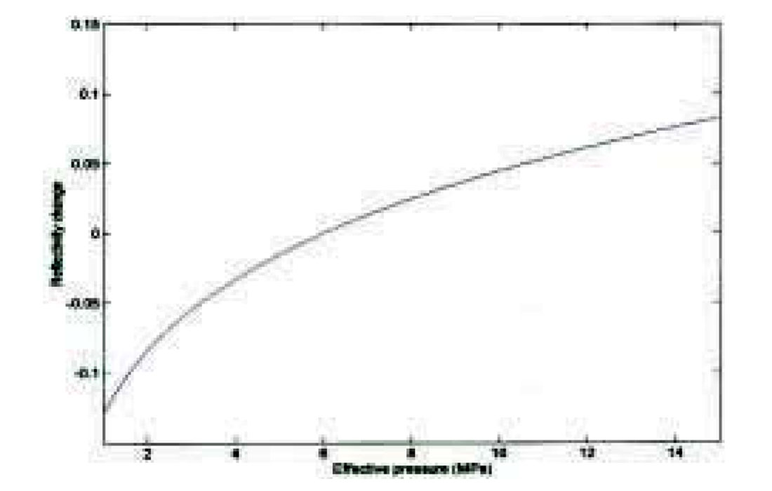
which means that according to the Hertz-Mindlin model the relative change in P and S-wave velocity should be equal. Ultrasonic core measurements done at core samples from some of the North Sea sand reservoirs indeed show that the relative changes in P- and S-wave velocities are fairly similar. However, comparison with dry core measurements often show that the exponent in equations (7) and (8) should be chosen closer to 1/10 rather than 1/6. Recent experiments done by Nes et al performed on artificial sandstone indicate that this exponent is less than 1/10. Figure 1 is an attempt to illustrate the uncertainty in determining velocity versus pressure curves. In this figure the results of Nes et al is sketched on the basis of their publication, and does not represent the real measurements.

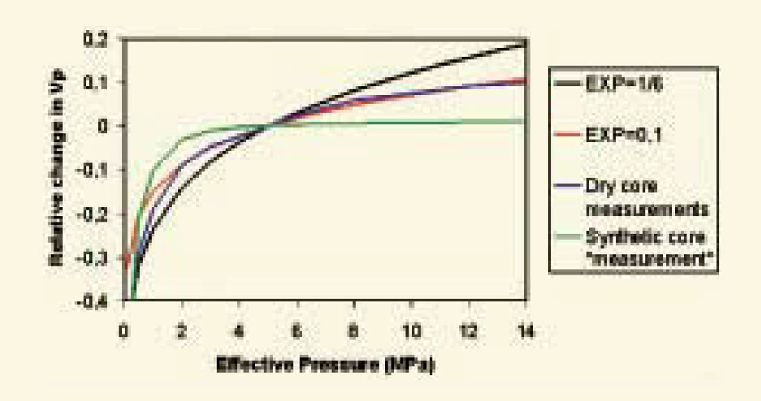
The key message from this section is that there are large uncertainties associated with the establishment of the velocity versus pressure curves. These uncertainties are multi-causal: up-scaling issues related to ultrasonic core measurements (are the rock physics measurements representative at seismic frequencies?), the coring process itself (as discussed by Nes et al), the unknown internal deformation coefficient (equation (3)), variability in core sample quality and so on. Therefore, alternative ways of estimating the velocity versus pressure curve is highly desirable, and in the present paper I will show some attempts to use the reservoir itself as a laboratory for obtaining such additional information.

Simple equations for overpressure detection based on Hertz-Mindlin theory

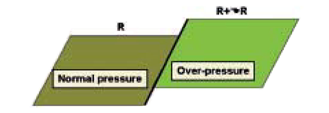
In the previous section it was shown that the relative changes in P and S wave velocities were the same for pressure changes. This observation can be used to derive simple equations relating the change in reflectivity due to changes in pore pressure. Figure 2 illustrates a situation of a fault acting as a pressure barrier between two segments.

A simplified expression for the PP reflection coefficient versus incidence angle can be written (Smith and Gidlow, 1984):

where Θ is the density and η is the incidence angle, and ΔV_P etc represents the change in P-wave velocity across the interface. For crystalline rocks, it is often assumed that the porosity and hence, the density changes caused by pressure changes are small, and thus we will assume zero changes in density across the sealing fault. The change in reflectivity across the fault barrier (Figure 2) is therefore given as

where Δ^V_P P and ΔV^S_P denote change in P-wave and S-wave velocity caused by pressure changes, respectively. Using equations (7) and (8), assuming an average V_P to V_S ratio of 2 (for shallow depths this ratio can be significantly higher), and further assume that sinΘ ∼ tanΘ we obtain

Finally, by inserting equation (7), a direct relation between reflectivity change and effective pressure is obtained:

This means that the change in reflectivity between the normal pressured segment and the over-pressured segment has a weak AVO-behavior (slight changes with offset), given that the V_P to V_S ratio is around 2. In addition to conventional velocity estimation for overpressure prediction, the simple formula given above can be used in a semi-quantitative way to identify potential abnormal pressure segments. Notice that for a pore pressure increase, the effective pressure, P, is decreasing, resulting in a negative change in reflectivity (equation (12)), as illustrated in Figure 3.

Fluid effects

In an exploration setting, one major challenge is to distinguish between pressure and lithology changes between the two segments shown in Figure 2. However, if we assume that the lithology is the same for the two segments, and assume that the segment to the left is water-filled and the segment to the right contains hydrocarbons, the change in reflectivity can be written as (see Landrø, 2001):

For many sand reservoir rocks, the density change is less than the velocity change, so a (very rough) approximation for the reflectivity change caused by fluid change is

This means that a fluid effect and a pressure effect has opposite AVO-effects, a light increase for fluid changes, and a slight decrease for pressure changes, as shown in Figure 4.

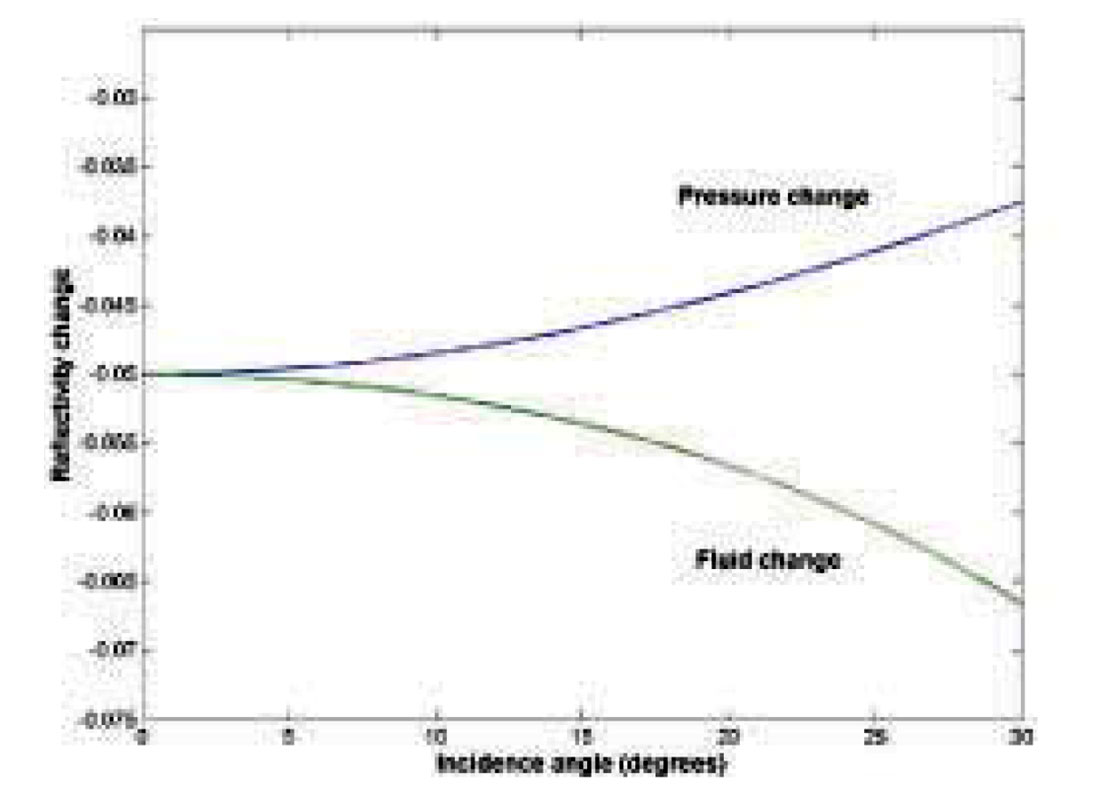
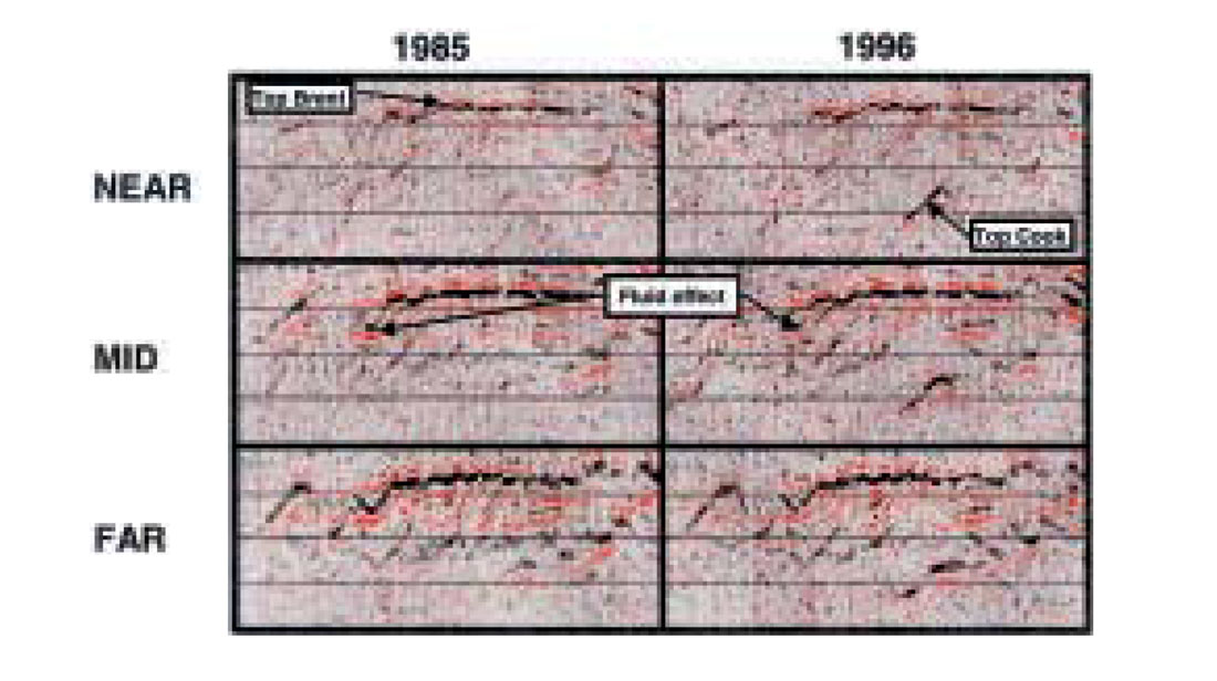
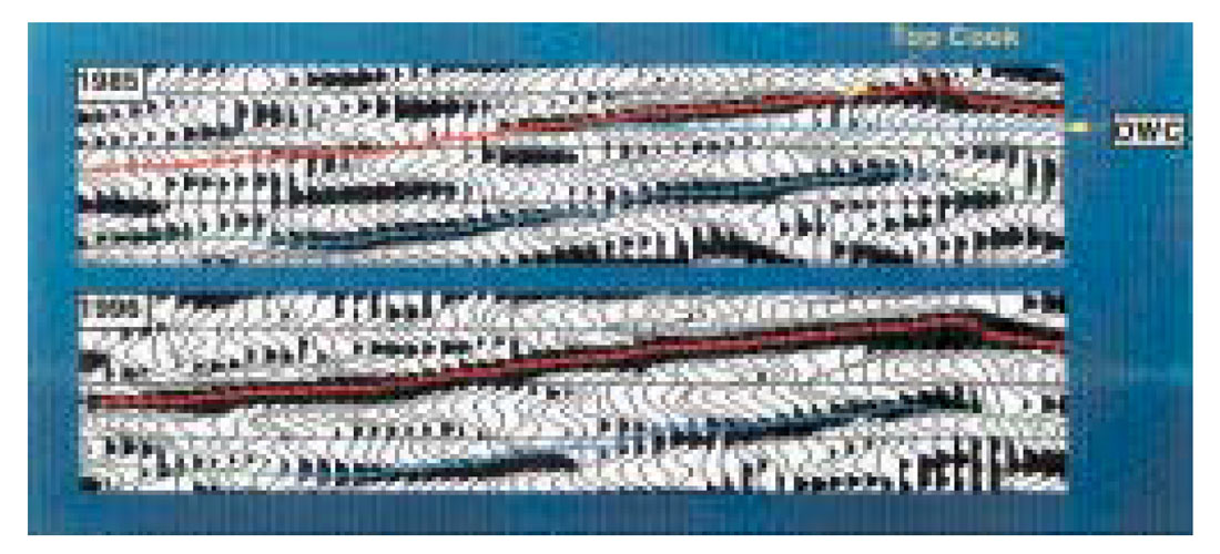
In Figure 4, the zero offset reflection coefficients have been chosen to be equal (or normalized to each other). The main limitation of this method is of course that we assume that the seismic parameters do not change significantly between the two segments sketched in Figure 2. A real data example, taken from a 4D case study is shown in Figure 5, where we can observe a slight amplitude decrease with offset after a pressure increase within the Cook Formation. Furthermore, we observe a slight amplitude increase (best visible on the near and mid offset stack, not so convincing from mid to far) with offset for the fluid marker at the 1985 data. In an exploration case, the uncertainty associated with a similar interpretation technique based on Figure 4 is much higher.

PS-converted data

A simplified version of the PS reflection coefficient is given as (Aki and Richards, 1980)

Following the same procedure as in the previous sections we find that for a pressure change, the corresponding PS reflectivity changes by (assuming a V_P to V_S ratio of 2)

For fluid changes we find correspondingly

This means that the PS-reflectivity changes have (to the lowest order) the same AVO-behaviour. The sign of the parameter contrasts depends on whether we are considering a pressure increase, a water to hydrocarbon fluid change or vice-versa.

A 4D example: Velocity changes caused by a pore pressure increase

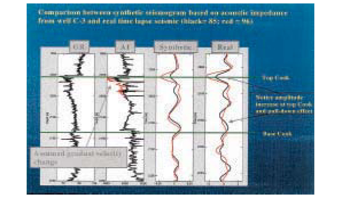
Figure 6 shows a time-lapse seismic profile from a segment where the reservoir pressure has increased by approximately 6- 8 MPa between the seismic surveys. A significant amplitude change is observed at the top reservoir interface. A detailed discussion of this case can be found in Landrø et al, 2001. There are significant variations in the size of this amplitude increase. A simple 1D modeling study based on well logs indicate that a P-wave velocity drop of at least 20% is necessary to explain the observed amplitude increase. This is illustrated in Figure 7. The reservoir thickness is approximately 80 m within the over-pressured segment. If a 20% velocity reduction is imposed for the whole reservoir thickness, a corresponding time-shift (or time-delay) of 20-30 ms should be observed on the time-lapse seismic data. This is however not the case, and therefore a gradual velocity change has been suggested in Figure 7. This gradual velocity change is to some extent supported by the increase in the gamma-log versus depth within the reservoir section (Figure 7). Although this time-lapse experiment is not a proof that the velocity should drop significantly for a pore pressure increase, it gives support to all the four curves displayed in Figure 1. As the number of time-lapse seismic surveys is increasing we think we will see more and more examples of this kind, where seismic velocities can be coupled to observed pressure changes within the reservoir. In most case examples there are limitations caused by reservoir heterogeneity, fluid and temperature changes taking place at the same time etc.

What about seismic effects caused by pore pressure decrease?

In the Gullfaks 4D seismic study (Landrø et al, 1999) several examples of pore pressure increases were found. The opposite effect, a pore pressure decrease, was not found, however. Even in areas within the water-zone where the measured pore pressure decrease was of the order of 2-4 MPa, no clear anomalies were observable on the 4D seismic data. The repeatability level of the Gullfaks 4D data was rather low, of the order of 50-70 % in RMS difference between baseline and monitor surveys. Last year, a dedicated experiment was done at Gullfaks, in order to further test the possibilities of detecting a pore pressure decrease (Landro et.al. 2002). A 12-level VSP tool was installed in one well, while a neighboring injector well was shot down in order to generate a pore pressure drop. The measured pore pressure decrease was 2.5 MPa. Although the analysis of the results of this test is not finalized yet, it seems clear that the effect on the 4D VSP data is rather small. One might therefore say that this “controlled” experiment, together with the 4D observations on this field, gives us a strong indication that pore pressure decreases are far less observable on 4D seismic data, compared to pore pressure increases.

Conventional velocity analysis, is it accurate enough to detect a pressure increase of 6 MPa at 2000 m reservoir depth?

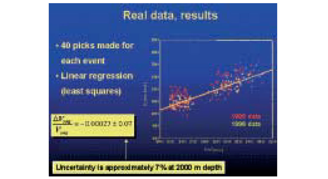
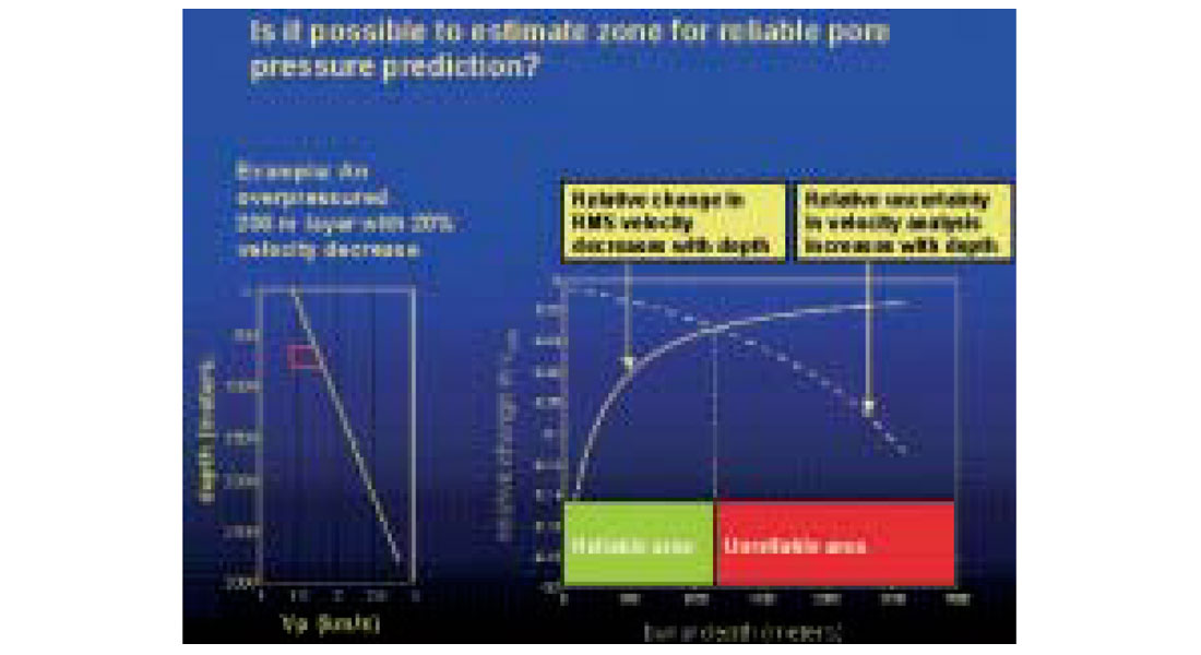
The example presented above can also be used to cast some insight into the sensitivity problem of using conventional velocity analysis for overpressure prediction. A thorough velocity analysis has been performed by Øyvind Kvam. He analyzed 40 CMP-gathers before and after the pressure increase, and found that the uncertainty in the velocity picking was larger than the estimated velocity change based on the velocity analysis. This is shown in Figure 8. There are several possible explanations for this, the major is probably the gradual velocity change mentioned in the previous section. The thickness and the depth of the over-pressured unit are crucial factors strongly impacting our ability to use velocity analysis as a tool for pressure prediction. The sensitivity for detecting abnormal velocity changes decreases rapidly with depth, while the uncertainty in velocity estimation increases rapidly with depth. This is illustrated in Figure 9. It is important to underline that the velocities displayed in figures 8-9 are RMS-velocities and not interval velocities as discussed in the previous sections.

Discussion

New simple AVO-formulas shows that the AVO-difference between a normal segment and a anomalous segment (over-pressured or hydrocarbon-filled), is opposite for a pressure effect compared to a fluid effect. These AVO-formulas are based on the Hertz-Mindlin theory, which predicts that the relative change in P-wave velocity is equal to the relative change in S-wave velocity when the rock pressure is changing. For some sandstone reservoirs, ultrasonic core measurements support this assumption (from Figure 3 in Landrø et al, 1999, we observe that the relative change in P- and S-wave velocities are around 4% for a 4 MPa decrease in net pressure, and approximately 10% for a 4 MPa increase in net pressure). It should be stressed that this assumption is based only upon the Hertz-Mindlin model and some rather sparse core measurements. Therefore, these simplified AVO formulas should be used with care for other rock types. Another limitation is of course that it is assumed that the lithology between the two segments (see Figure 2) is constant. A relatively small change in lithology between the two segments might of course mislead the AVO-interpretation technique suggested in this paper. Therefore, it is important that the suggested method is regarded as complementary to the more established pressure prediction methods, based on velocity analysis.

Time-lapse velocity analysis applied on a “controlled” overpressured segment demonstrates clearly two critical factors: thickness and depth of the over-pressured layer. The uncertainty associated with our pressure predictions increases rapidly with depth, and decreases rapidly with the layer thickness.

Conclusion

Recent 4D seismic case studies show that pressure effects are visible and detectable as 4D amplitude differences. There are also strong indications that pore pressure increases are easier to detect than pore pressure decreases. This observation is in agreement with most ultrasonic core measurements. Based on the Hertz-Mindlin theory it can be shown that a pressure anomaly has the opposite AVO-behavior (decrease) of a fluid anomaly (increase). This simple observation can be used as a complementary interpretation technique for identification of over-pressured segments. 4D seismic has also shown that seismic amplitudes are robust, often more robust than travel-time differences. Correspondingly, we should put more emphasis on the use of amplitudes (and AVO) also for pressure prediction in an exploration setting.

Acknowledgements

Statoil and the Gullfaks licence partner, Norsk Hydro are acknowledged for permitting this paper to be presented. Martin Landrø acknowledges financial support from the EC project ENK6-CT-2000-00108, ATLASS. Alexey Stovas is acknowledged for comments to the manuscript.