On Calibrating Curvature Data to Fracture Density: Causes

Summary

Volume curvature attributes have been used to infer fracture density in a variety of seismic data worldwide. Estimating accurate quantitative fracture density values from curvature data is of special importance because curvature belongs to a general class of attributes that infer fractures through causal relationships rather than through direct detection of them. This does not necessarily make curvature of greater or lesser use in our efforts to understand fractures, but rather adds a special perspective to strategies around its calibration. Beyond the obvious general utility of producing measureable numerical values, estimates of fracture density variations may be useful in assessing completion and production opportunities and risks. Calibrating curvature data extracted from 3D surface seismic data to actual fracture density values is unlikely to ever be a trivial task. This calibration will require both the acquisition of appropriate control data such as image log data, core data, and cross dipole log data. The sample size of this control data is unlikely to be generally sufficient to fully calibrate most of the curvature data by itself. We must bring forward geologic knowledge of the causes and behavior of fracture development to constrain our calibration and provide perspective to the sample data we do have. In particular, we must be aware of the effects of the fractured reservoir’s material properties, in-situ properties, and structural position. We will also have to consider other fracture inferring and detecting methods and find practical combinations with curvature that utilize the various attributes’ connection to the causes of fractures as well as their circumstances of validity. The most practical opportunities for meaningful- although probabilistic- fracture estimation will likely come from the use of all available calibration data, a leveraged use of a variety of prediction attributes and a strong understanding of causal variables.

Introduction: Question from the October 2009 Luncheon

At the end of the October 2009 CSEG technical luncheon, the question was posed as to how curvature attributes could be used to infer actual fracture densities. To be efficient with time, the statement that “Curvature may infer fracture variation” had been shortened to “Curvature predicts fractures”. In reality, it might be more correct to say “infer” than “predict” since curvature does not directly detect fractures. That being said, we do use curvature attributes as a predictor of fractures. The missing step in prediction is calibration to actual fracture density values. As small a step as calibration may seem to be- only as significant as the difference between the words infer and predict- the act of calibration is in no sense an easy one.

There are many different attributes that are used in the effort to predict or infer fractures. There are commonalities in the calibration of any and all of these attributes, but also some differences. These differences are related to the connection the attribute has to fractures. Some attributes, such as azimuthal AVO and azimuthal velocity analysis are direct detection methods. These methods have physical criteria that must be met in order for their methodologies to be valid. For instance, some small angle applications of Ruger’s equation require that fractures be nearly vertical and in similar azimuthal alignment (Goodway et al, 2006). There are variations on this class of method that may have greater flexibility. A discussion of these methods is beyond the scope of this short note, but it is worth pointing out that for these methods, we must understand something about the nature of the fractures, their orientation, and likely variation. We have chosen to delve deeper into curvature methods in this note simply out of interest born from the recent CSEG luncheon question. Curvature methods are related to fractures through their representation of strain in the earth (Nelson, 2001). Strain is one of many causes in the development of fractures and their variation. Since curvature does not directly detect fractures, but is causally related to them, calibration of curvature requires an understanding of stress, strain, and the other causal variables of fractures. The work of calibrating curvature to fracture density thus requires that we understand more about fractures, how, and why they form.

Calibration to fracture densities requires the combined use of physical knowledge of fracture causes and behavior with control data. Ronald Nelson (2001) published an exemplary work called Geologic Analysis of Naturally Fractured Reservoirs. Nelson’s book is a milestone in terms of collecting previously published studies, laboratory, and field data on the behavior of fractured reservoirs. Nelson’s description of the causes of fracture development is comprehensive, but is not geophysically focused. Our short note essentially applies and describes Nelson’s principles to the calibration of 3D seismic curvature data. We recommend further that interested persons read Nelson’s book, which we have borrowed heavily from. In no sense is this note comprehensive, and we must admit that generalizations are used liberally throughout this note. This has been done in the hope of capturing at least enough of a flavor of the key elements to be considered in curvature based fracture prediction and calibration that the oil and gas explorer has a starting point from which to attack the problem in greater detail.

Many Kinds of Fractures

Fractures are a kind of deformation in the rock as a result of stresses on that rock. The present-day fractures are formed as a result of the total stress history that a rock has undergone, i.e. the history of the stress field as well as the physical changes that the rock has undergone as it is buried and gets consolidated/ compacted. The present-day stress field is a combined action of the tectonic stresses in the area, the overburden pressure, the pore-fluid pressure, local stress effects, and the material rock properties among other things. So any attempt at prediction/ inference of fractures would need complete details of such processes and their understanding as well as how the present-day shapes are related to them, which is not always an easy task. To break the daunting problem of understanding and predicting fractures into more easily dealt with components, we could start by considering the main classes of fracture systems we are likely to encounter in oil and gas exploration and development, the types of compressive fractures we will likely encounter, and the morphology of the fractures themselves.

Classes of Fracture systems

Geologically, fractures may be divided into many classes, with the two main classes of oil and gas significance being regional and tectonic. Regional fractures are predictable in behavior and while they develop over large areas, they seem to occur over a smaller range of scales (they may not exhibit fractal behavior). Regional fractures have very small variance in orientation and density and are typically not densely spaced. Regional fractures are commonly set up with orientations in alignment with the long and short axis of the local basin they are found in. They are less well understood, with several schools of thought as to how they are formed. One notion is that regional fractures are formed as a result of crustal forces, while another is that they are caused by basin compaction forces that are developed basin-wide.

Tectonic fractures are formed in response to the area tectonic stress field and local tectonic events such as folding or faulting. These fractures appear at an incredible variety of scales, and are commonly considered to be fractal in nature. Tectonically related fractures often have a similar orientation in an average sense, but may also have wild local variations in orientation and intensity as the rock deforms. Fractures may arise due to the folding process itself. Fractures due to faulting are formed as a result of area wide stresses that instigated the faulting, and are commonly clustered in shear conjugate halos about the fault plane. Fractures formed due to folding are often associated with hydrocarbon production and so are of interest. In fact, the fracture type that we tend to see in 3D surface seismic curvature data is tectonically related.

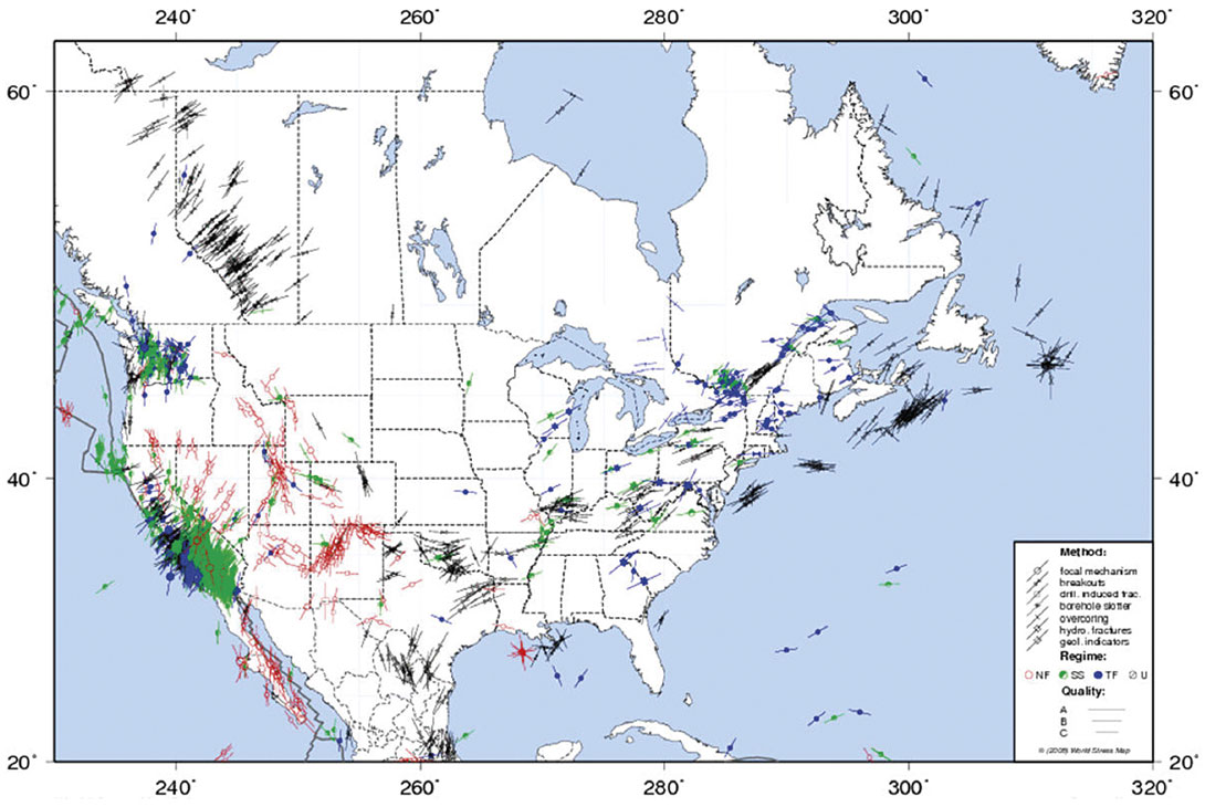
Figure 1 illustrates the main mapped fracture systems in North America. Interestingly, although this map is clearly regional in scale, the fractures being mapped are likely both regional and tectonic in origin.

Stress, strain, and compressive fracture types

Regardless of the type of fracture system, all fractures are caused by stress. Application of stress at any point on the rock induces strain, which is a measure of the change in the shape of rock as a result of the application of stress. For mild stress levels, the deformation of the rock is elastic, and the rock will recover its original shape when the stress is removed. The relationship between stress and strain is linear and governed by Hooke’s law. For higher stress levels (greater than the elastic limit of rock), the deformation of the rock results in brittle failure and fracture. Fracturing, faulting, folding, and other types of deformation are all responses that alleviate the stress applied to the rock.

In general, the three-dimensional (tri-axial) stress field can be resolved in three orthogonal principal axes of stress, denoted by σ₁, σ₂, σ₃ as shown in Figure 2 . σ₁ is for maximum, σ₂ for intermediate and σ₃ for minimum normal stress.

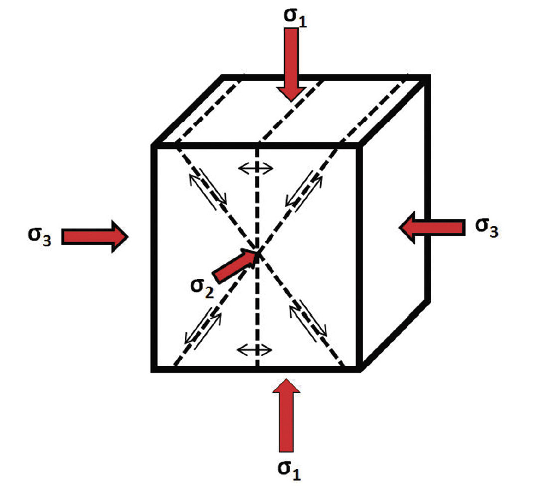
The shear fracture planes are at acute angles to the maximum compressive stress direction. We may also encounter another type of compressive fracture, called extension fractures, which will be oriented parallel to the maximum compressive stress. If the maximum compressive stress is vertical into the earth, the extension fractures will then also be vertical, and the shear fractures will be at an acute angle to vertical. Deep, mildly folded targets will often be dominated by these type of fractures, although the direction of maximum stress may change depending where on the fold we are looking. Shear fractures will also commonly occur in a halo about faults, in orientations at acute angles to the fault plane.

Since σ₁ is often perpendicular to the earth’s surface for targets at sufficient depth, the natural fractures we encounter in the pursuit of oil and gas may be sub-vertical to vertical depending on depth. There are exceptions to this situation, such as for shallower targets, for certain positions on some folded structures, and for some strike slip faults where the maximum horizontal stress is greater than the vertical stress. Assessing the stress field may be important in considering the validity of other fracture detecting attributes such as azimuthal AVO analysis. Curvature is a key indicator from which the current, local, strain is illustrated.

Fracture morphology

Fractures may be classified according to morphological descriptions such as: open (uncemented with no change to the original fracture surface), mineralized (which may be partially open), deformed, or vuggy (formed as a result of acidic water percolating through fractures). The effect that fractures may have on completion and production behaviour depends heavily on their morphology, so an understanding of what kind of fractures may be present is critical. Open fractures typically have very high permeabilities in the direction parallel to the fracture orientation, with permeability being related linearly to fracture density and to the cube of the aperture width of the fracture (Parsons, 1966). Mineralized fractures are often partly open and can have a wide range of permeability. More information on Fracture classification and morphology is found in Nelson’s book.

Whether the fracture morphology is going to be open, mineralized, deformed or vuggy depends heavily on the rock brittleness, and the history of burial, paleo-stress, and in-situ conditions such as pressure, rate of deformation, and diagenetic factors. Although we may encounter any general type of fracture, for our Western Canadian Sedimentary Basin, we commonly encounter fractures caused by compressional stresses, particularly shear fractures. Another thing to keep in mind is that we are most concerned with open or (more likely) partly open fractures here, as it is these types of fractures that have a bearing on the flow capacity of the reservoir. These morphologies are also most likely to be seen on AVAz attributes, although completely filled fractures and deformed fractures may have an anisotropic effect on seismic as well, depending on the infilling material.

Causes of Fracture Density Variation

While there is great utility in considering the nature of the fracture system, as well as the type and morphology of the fractures, we eventually must consider the proximate causes of fracture density variation. Fracture density will always be predicted from curvature in a probabilistic fashion rather than a deterministic one because of the many proximate causal factors at hand (some or many of which we cannot perfectly determine) and the fact that the real earth has variance. Nelson describes the main causes of fracture density variations. Those causes are summarized in Table 1 below:

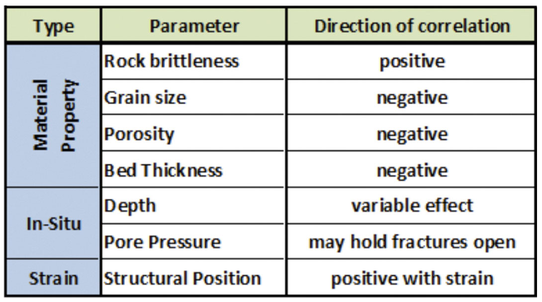
The implications of these causes are many, some of which are intuitively obvious. It is clear then, that one cannot simply look at a curvature map and suggest- from the curvature data alonewhat the fracture density variations might be. The variations will depend on changes in the rock brittleness, as well as other factors illustrated in Table 1. For example, curvature values shallow in the seismic section will likely infer a very different fracture density from the same curvature values much deeper in the section where the rock brittleness and vertical stress could be vastly unalike. Nelson discussed one case study of a folded outcrop in his book where the change in fracture density was greatest going from the forelimb to the hinge zone for a less brittle limestone than a more brittle dolomite, even though the more brittle dolomite had a greater overall fracture density. According to the field and laboratory work compiled, reservoirs with the same curvature values would relate to rocks with different fracture densities depending on whether they were a thin bedded quartz rich sandstone versus a massively bedded sandstone, or a limestone versus a dolomite, or an clay rich shale versus a quartz rich shale.

None of these comments suggest we should not use curvature as an important tool in our efforts to predict fracture density variation. We should use curvature: it is a robust tool that can give profound information on strain in the rock. The point here is that we must also consider these other causal variables in our calibration.

Calibration (or control) data

A serious challenge in the calibration of curvature to fracture density is acquiring a sufficient sample statistic of control data. There are many sources of calibration data, some of which may be recorded in vertical wells, some in horizontal wells, and some in both kinds of well. Each of these approaches has different costs, measurement method, accuracy, and (depending heavily on the kind of well it is recorded from) sample size and the orientation of fracture that is likely to be encountered.

• Full core analysis
• Downhole cameras
• Image logs
• Microseismic data
• Shear wave polarization observed in VSP
• Shear wave polarization observed in crossed dipole full waveform recording in vertical wells
• Stoneley wave analysis

Fracture density has an unusual requirement of a large sample statistic because we must measure changes in the density of fractures, and thus simple point measurements will be insufficient. Although fractures may be observed in vertical or mildly deviated wells, the lateral size of the data being sampled in such wells remains very small, particularly for an attribute such as curvature which requires formation by formation calibration (as explained above). Single vertical wells may miss entirely nearby swarms of fractures simply by chance and give misleading calibration information. This is not to say such data has no use, only that we desire a significant amount of it.

Crossed dipole anisotropy data or whole core analysis may yield fracture density information in vertical or mildly deviated wells. One advantage of this information is that it can be used to observe differences in the fracture density seen in a variety of formations, even if we have some reservations about its sampling. A very desirable type of data is fracture density, angle to the vertical, and azimuth observed in image logs such as Full Bore Micro Imager (FMI) logs. This log can observe very small fractures and can be used in vertical or horizontal wells. Continuous lateral fracture density data from image logs recorded in horizontal wells can provide bigger sample statistics to calibrate curvature observations.

Ideally, we would have a variety of fracture density or anisotropy control data from a collection of vertical and horizontal wells so that we could calibrate and compare the fracture densities at more than one formation.

Curvature

Curvature is a structural position, or strain related fracture density method that has been used by geologists since the late 1960’s. As Nelson describes below, the curvature method infers fracture density based upon three assumptions:

1. The rock is brittle and fails largely from fracturing
2. An increase in curvature implies an increase in strain
3. An increase in strain implies an increase in fracture density

These observations are well supported by geologic studies of fracture densities measured at various points on folded features, although reference to the other causes of fracture density variation (Table 1) are also required for quantitative calibration. Nelson describes how areas of maximum curvature identify the all important hinge zones of folded features.

Smaller scale features must also be considered. Sufficiently large scale folds and faults may be readily observed on seismic reflection data. Curvature is useful in specifically identifying the hinge zone of these larger features, but its value may be greater for smaller scale features that are not so obvious of reflection data. Figure 3 shows a chair display with the most positive curvature on the horizontal display (horizon slice) and seismic on the vertical. Notice the smaller features seen on the curvature display are associated with undulations on the reflections. These small features could have a multitude of causes such as stratigraphic changes, small bends or folds in the rock, smaller scale faults that do not exhibit observable breaks in the seismic, or even zones so broken that the wavefield is scattered. Curvature attributes may pick up these signatures and exhibit them as lineament patterns. Stratigraphic variation including bedding or other depositional morphology may be observed as lineaments in curvature or other discontinuity and shape related attributes. This can be a source of error in fracture inference if not considered. The other factors that create these small scale curvature features are all deformation related, whether by strain where the rock is folded, or through faults. Any of these features have causal relationships with fractures. In consideration of these many direct and indirect causal relationships, our motivation to statistically calibrate the observations to control points is reinforced.

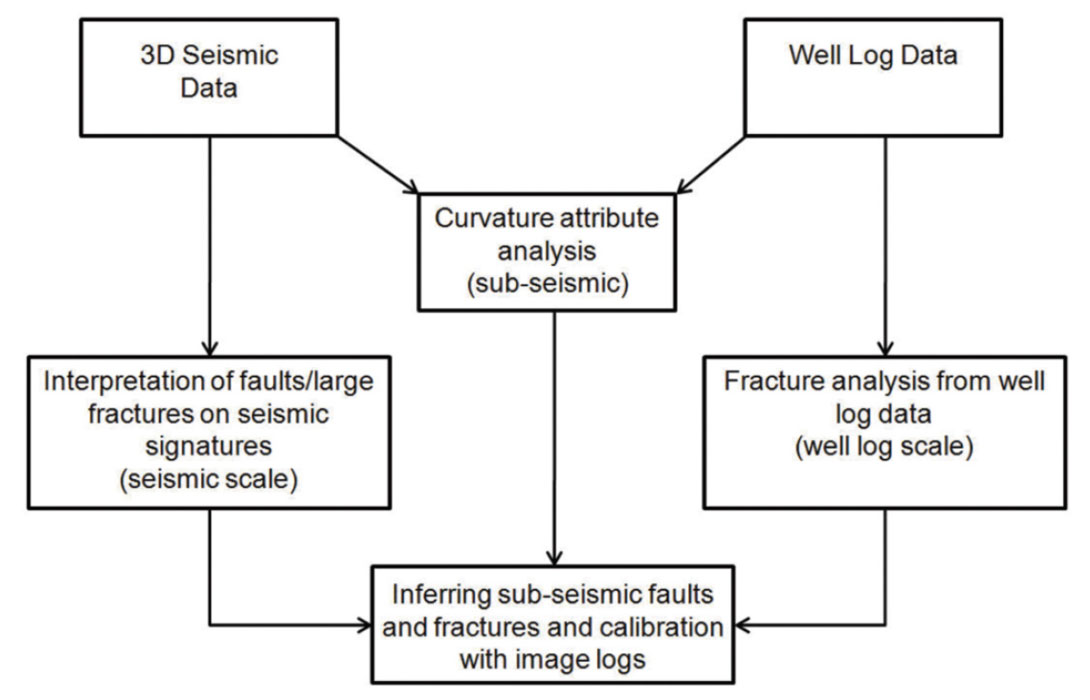
What we need is a workflow that is in-between the small-scale well data scheme and the large-scale seismic data. To this end, the flow diagram shown in Figure 4 outlines the procedure we follow for a method that makes use of curvature attributes and their calibration with well log data to infer about fractures. There have been some studies in the literature where calibration efforts have followed procedures similar to the one we illustrated in Figure 4. These studies have shown that in various fractured reservoirs higher values of curvature have been found to be correlated with increased occurrence of fractures (Lisle, 1994). Narr (1991) related increased fracture density to the location of a doubly plunging fold hinge in Point Arguello oilfield in California. Similarly, Ericsson et al (1998) who defined a strong relationship between fracture density and curvature for the Fateh Field, offshore Oman.

Practical considerations

The advent of sophisticated and robust curvature measurement from 3D seismic volumes has provided a unique opportunity to use this kind of fracture density inference over vast, continuous areas. Despite its strong need for calibration- and all fracture density estimators require some calibration- curvature has some inherent advantages as a fracture density estimator:

• Curvature is computationally cheap to produce
• Curvature is calculated on stack data, and is hence more robust than many fracture density estimators
• Curvature has no requirement regarding fracture angle or alignment

This is not to say that curvature competes with other methods such as azimuthal AVO fracture estimates. In fact, curvature methods are best used in conjunction with azimuthal methods. Fracture systems with no apparent measured structure may be missed by curvature methods just as some applications of azimuthal AVO methods may fail if fractures are not nearly vertical or in near uniform azimuthal alignment. There will be places where either situation may occur. Since there are many types and behaviors of fractures coupled with a multitude of proximate causes of fracture density variation, we must neither believe any one method too certainly nor should we discard another too quickly. Ultimately each method must be considered through an investigation into the physics it is based upon and its relation to the particular kinds of fractures expected in the area as well as with the all important calibration to hard control or calibration data.

Conclusions

As there are many different types of stresses possible, and many different rock types, there are therefore many different styles of deformation, and many different types of fractures. Nevertheless we do need to focus on the characterization of different types of fractures and faults in our reservoirs in terms of their density and orientation. These properties are then used as input to either generate or upgrade a reservoir model and study the bearing they have on reservoir production. In the absence of a complete understanding of the geological history of the area, characterization of fractures and the level of expectation from any technique or methodology adopted should consider the overall scenario.

Curvature is a valid method of inferring fracture densities through its connection to structural strain. The fact that curvature addresses one of many factors affecting fracture density means that we must both consider these other factors in a calibration of curvature data to quantitative fracture density, and that we must also acquire significant control data such as image log fracture density in horizontal wells. Curvature may have these heavy requirements on the road to quantification as a fracture density predictor, but it also has many practical advantages, and will remain- perhaps grow- as a tool in our understanding of fractures. It is hoped that we can use various fracture predicting techniques with curvature, as well as acquire what control data we can to move further from “inferring” and get closer to “predicting”.

Future Work

At GeoCanada 2010, Fairborne Energy, CGGVeritas Canada, and Arcis Corporation will present a combined effort where we demonstrate a case study involving the calibration of curvature and AVAz attributes to fracture density and produce estimated fracture density maps.

Acknowledgements

We would like to thank Jon Downton of CGGVeritas for various discussions as well as Arcis Corporation for permission to use the data example in Figure 4.