Offshore East Coast: Model-based Water-Layer Demultiple Breathes New Life into Old Data

This article describes recent development and application of a model-based water-layer demultiple technique. We discuss some application details such as the water-bottom Green’s function and the necessity of a two-step prediction to handle both shot-side and receiver-side multiples. This method is tested using a finite difference synthetic dataset and then applied to two different 2-D marine lines from offshore East Coast of Canada.

Introduction

A recently announced discovery has brought renewed attention to the potential reserves in the Canadian Atlantic waters, complementing the huge reserves onshore in the Western Canadian Sedimentary Basin. According to Reuters “Statoil said its Bay du Nord find, around 500 kilometers (300 miles) northeast of St. John, could contain between 300 million and 600 million barrels of recoverable oil.” (Sep 26, 2013).

This is therefore an opportune time to take a look at one of the key issues for making best use of seismic data when mapping these reservoirs: the attenuation of problematic water-layer multiple energy. The variation in water depth from a few 10s of metres to several 100 metres poses a special challenge, as not all multiple attenuation methods work equally well in these different situations.

Surface Related Multiple Elimination or SRME (Verschuur et al., 1992) has become the de facto standard for marine demultiple. SRME is based on the prediction of multiples by convolving the data with successive estimates of the primaries in a recursive estimation procedure. It has been demonstrated repeatedly to be effective for both 2-D and 3-D multiple attenuation, in moderate to deep water. However, it is well recognized that SRME can struggle with shallow water multiples, especially in the presence of a hard water bottom. The main reason for this is that these water-layer multiples can have significant amplitudes up to high orders, where the “order” of a multiple refers to the number of downward bounces from the sea surface. The peg-leg multiples from deeper events often lie close to water-layer and shallow peg-leg multiples of high order, that are relatively over-predicted by SRME. This leads to the failure of any adaptive subtraction procedure to simultaneously match all orders of multiple. Moreover, accurate prediction of the water-layer multiples, requires primary energy at very near offsets which are typically not recorded.

For this reason a new breed of demultiple algorithms has been developed for shallow water, known variously as: “Deterministic Water-layer Demultiple”, or DWD (Moore and Bisley, 2006); “Model-based Waterlayer Demultiple”, or MWD (Wang et al., 2011); and “Shallow Water Demultiple”, or SWD (Wang et al., 2012; Yang and Hung, 2012). We prefer the abbreviation MWD, though care is needed to avoid confusion with another MWD: “Measurement while drilling”! In this article, we review the principles of MWD and report on our implementation of an MWD method based on diffraction modelling for the water bottom Green’s function. We demonstrate the application of MWD using a synthetic dataset and then using two different East Coast 2-D marine lines.

What is MWD?

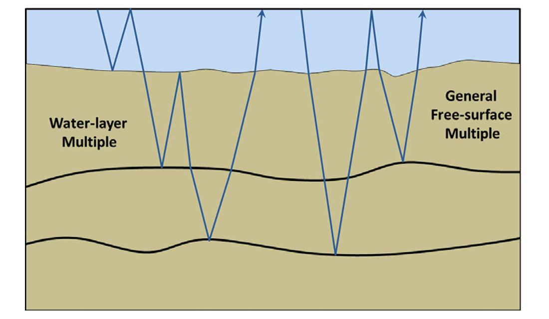
Figure 1 illustrates two different types of free-surface multiple. On the left is a water-layer multiple which is defined to be one which has at least one upwards bounce at the water bottom and one downward bounce at the surface. It is a special case of the more general free-surface multiple, which may or may not include an upward bounce at the water bottom. SRME addresses both of these types of multiples, but with limitations as outlined above. MWD on the other hand only seeks to attack the water-layer multiples and defers the remaining free-surface multiples for subsequent attenuation by an SRME type approach.

In Figure 2, we show two different orders of water-layer multiple. Each is constructed by combining the water layer Green’s function (shown in red) with a general ray-path (shown in blue), which represents events in the recorded data. Any higher order water-layer multiples will be predicted by the Green’s function applied on the previous order multiple which exists in the data. All orders of water-layer multiple are thus predicted by operating on the data with the Green’s function.

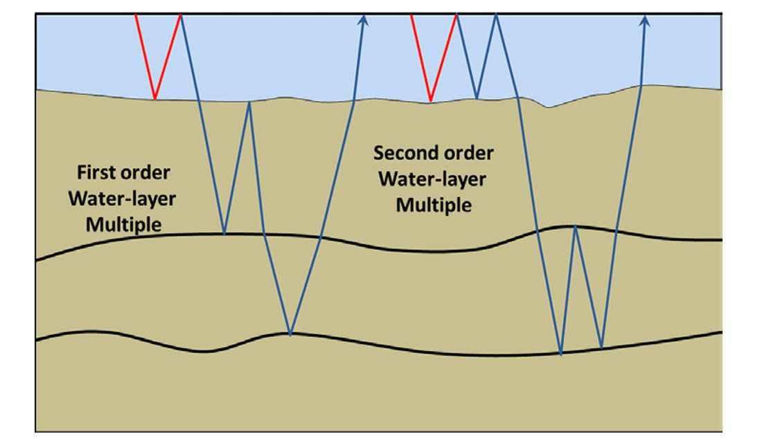
The prediction may then be subtracted from the data to obtain a water-layer multiple-free record. Note that shot-side and receiver-side multiples have to be separately dealt with, a topic we return to below.

We have used terms rather loosely above such as “constructed” and “Green’s function”. We will now expand a little on what this means, describing it for the shot-side multiple removal. Similar to SRME, the MWD method relies upon cross-convolution, in this case cross-convolution of the water-bottom Green’s function with the data. The Green’s function used is the wavefield recorded at various points on the surface due to an impulse generated at the shot, with reflection from only the water bottom. Various methods are possible for generating the Green’s function. For example, Wang et al. (2011) make use of wave-equation extrapolation operators. Our method uses diffraction-based modelling of the Green’s function from the interpreted seafloor.

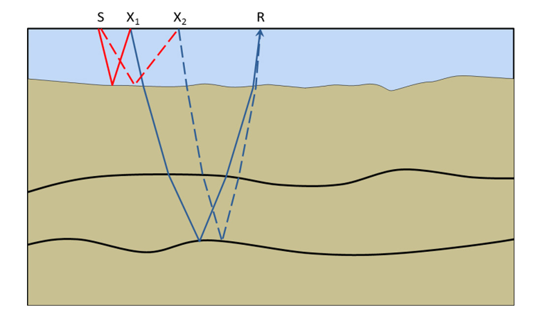
Given any input trace with shot position S and receiver position R, the water-layer multiples are then predicted by convolving the Green’s function from shot position S and receiver position X with the data from shot position X and receiver position R, where X is the downward reflection point (DRP) for the multiple. This is repeated for all sensible positions of X (based on aperture considerations), and the results are summed to produce our multiple estimate. This is illustrated for two such DRPs, X₁ and X₂, in Figure 3. Note that in Figure 3, position X₂ would correspond to a non-specular downward reflection for this relatively flat geology. However, this cannot be known a priori, and it might correspond to a specular reflection for some other dipping reflector. The MWD method relies on Fermat’s principle, such that the summation will naturally select the specular events by constructive interference and remove others by destructive interference.

For 2-D, the above multiple prediction is mathematically formulated in the frequency domain, ω, by the following equations, where s, r and x are coordinates for the shot, receiver and DRP respectively, D is the input data, G_wb is the water-bottom Green’s function, M_sht/rec are the shot and receiver side multiple estimates, and D_nw is the estimated data with no water-layer multiples:

EQUATION 1

for the receiver side, followed by,

EQUATION 2

for the shot side. Here D₁ is an intermediate result in which only receiver side multiples have been accounted for. It is important to use D₁ to predict the shot-side multiples rather than D, as use of D would result in the double prediction of any multiples which have both a shot and a receiver-side peg-leg.

This separation into shot-side and receiver-side operations is not widely discussed in the literature (an exception is Jin and Wang, 2012). However, as shown below, it is absolutely necessary in situations where the seafloor has structure.

Modelled Data Example

Figure 4 shows the model we have used for testing the MWD algorithm. Finite difference modelling was performed by a client, who provided us with the synthetic data. We particularly want to focus attention on the challenge posed by the rugose part of the water bottom from about 4km to 8km lateral position. The variation in water depth implies that shot-side and receiver-side peg-leg multiples are not spatially coincident, and require the two step methodology outlined above.

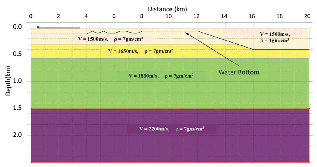
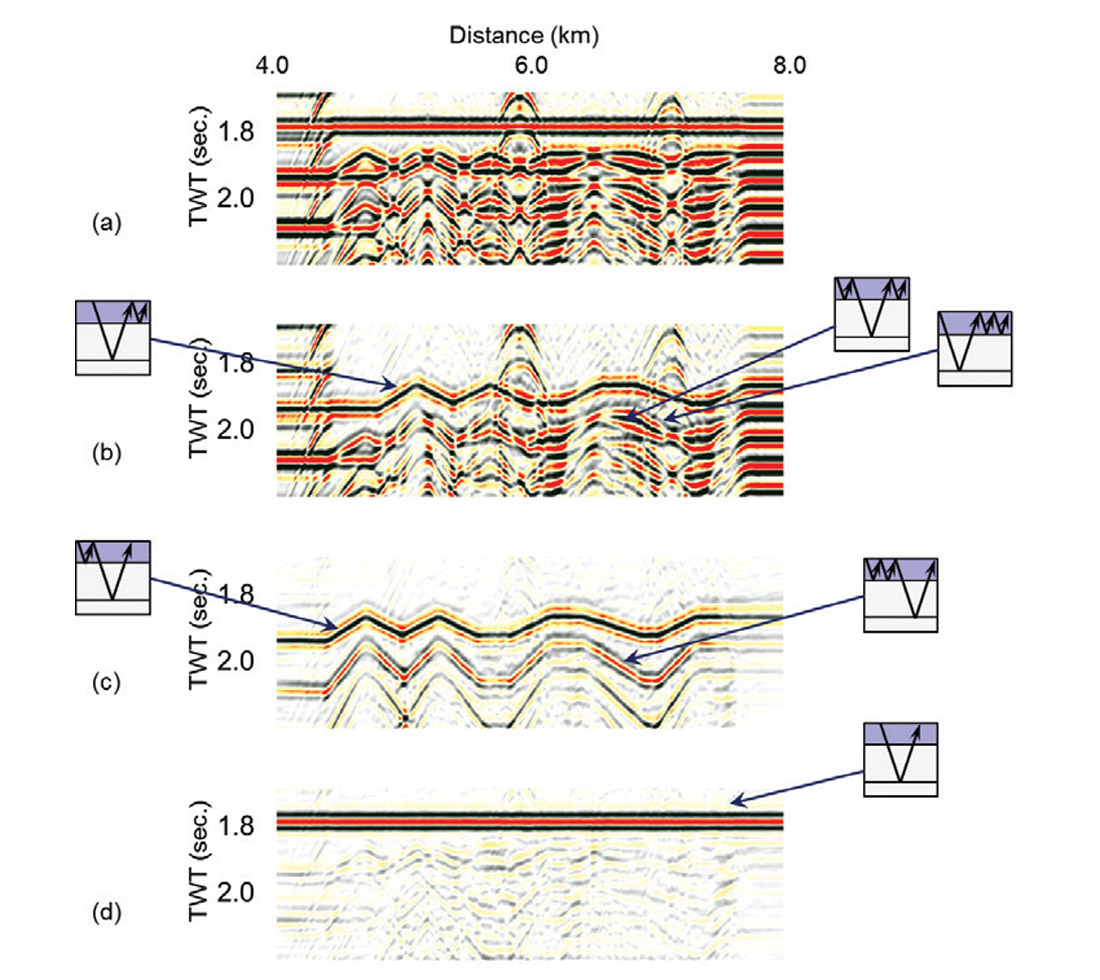
Figure 5 shows a stack of the modelled data before and after application of MWD. The area shown within the blue rectangle is considered in greater detail in Figure 6, which shows a constant offset section from the data (offset = 587.5m) and illustrates the steps of the MWD procedure. We focus attention on the reflection at a depth of 1.5km, for which the primary appears at about 1.8 seconds in Figure 6. The first order peg-leg multiples appear on the input data (6a) as two separate overlapping arrivals (at about 1.9 seconds) which have different imprints from the variable sea floor geometry above. One of these is predicted during the first step, the receiver-side demultiple in 6(b), whereas the second is only predicted in the second step, the shot-side demultiple in 6(c) (note that 6c includes the results from both shot-side and receiver-side prediction). Likewise for the three 2nd order peg-leg multiples (at about 2.0 seconds): two of them are predicted in the first step in 6(b), (because they both have receiver side peg-leg components), but the third is not predicted until the second step in 6(c). Finally we subtract the full set of multiples to obtain an estimate of the primary only data in Figure 6(d). The key point to note is that application of the Green’s function by convolution on either shot or receiver side cannot predict a multiple unless it has a water layer bounce on that side. Of the multiples identified here, only the symmetric 2nd order multiple can be predicted by either a receiver-side first or a shot-side first approach. In Figure 6, it is predicted by the receiver-side demultiple, simply because that is the first one applied.

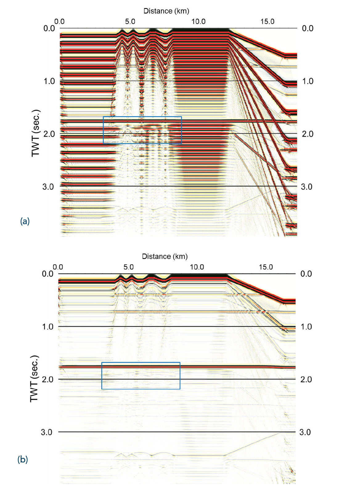
Returning briefly to Figure 5, the observant reader may have noticed a faint event below 3 seconds, which appears to resemble a mirror of the water bottom. This event is also a multiple, but not a free surface multiple. It arises from energy reflected from the interface at 1.5km depth, which hits the water bottom from below and bounces downwards before a second upward reflection. It is indeed a mirror image of the water bottom, with the event at 1.5km acting as the mirror! This multiple is a technically an internal multiple and would need the application of an internal multiple attenuation to remove it, beyond the scope of this article.

East Coast Canada 2-D Marine Data

We now demonstrate the application of our MWD method on two datasets from offshore Eastern Canada.

The first of these examples is a 2-D line from North Flemish Pass, provided to us by Jebco Seismic (Canada) Company. The data were acquired in August, 1998, with shot and receiver spacing of 25m and 12.5m respectively, with maximum offset of 6100m. Over the total length of the line the water depth varies from approximately 165m to 1200m.

Figure 7(a) shows the stack of the input data for approximately half of the line, predominantly in the shallower end. Figure 7(b) shows the result of subtracting the water-layer multiples predicted using MWD from the input data.

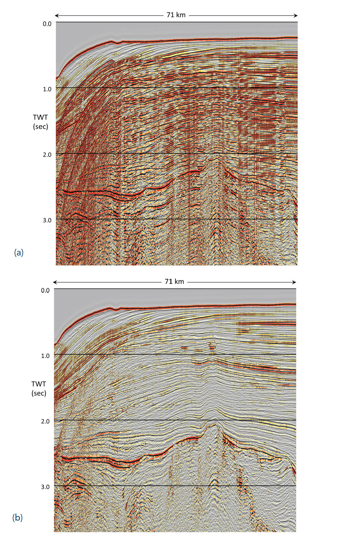
From approximately 0.5 seconds to 2 seconds in Figure 7(a) the primaries are obscured by several orders of water layer multiple, which are significantly attenuated by MWD in Figure 7(b). Furthermore, peg-leg multiples generated by the strong reflector at approximately 2.5 seconds are also well attenuated by the MWD.

The second example is another 2-D line from offshore Eastern Canada. The data were shot with shot and receiver spacing of 25m and 12.5m respectively, with maximum offset of 8230m. The water depth varies from approximately 100m to 420m along the line shown.

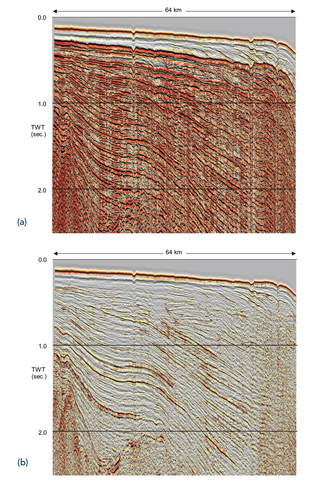
Figure 8 shows a comparison of stacks before (a) and after (b) application of MWD on this line. Again we observe that very strong multiple energy, which dominates the section from the first water layer multiple onwards, is significantly attenuated after application of MWD, allowing the previously obscured primary energy to become visible.

Conclusions

It can be worthwhile to revisit older datasets in the light of new technology. In this case, we have made use of recent advances in the understanding of multiple prediction and removal, especially for shallow water-layer multiples, to attack problematic multiples on 2-D marine datasets. We have adopted a diffraction modelling approach for generating the Green’s function, for use in the MWD algorithm, which we have then tested with some quite challenging synthetic data. One lesson from this was the importance of separately handling shot-side and receiver-side peg-leg multiples, to properly deal with structure, especially variation in the water bottom. Application of MWD on two different 2-D marine lines produced what seem to be more coherent and geologically plausible sections.

Acknowledgements

The authors wish to thank Key Seismic for supporting the publication of this work.

We thank an anonymous client for provision of the modelled data used in this paper.

We thank Jebco Seismic (Canada) Company, owner of the North Flemish Pass data, for permission to show the first field example in this paper.

We thank two anonymous clients for permission to show the second field example.

We would also like to thank Jeff Deere for his meticulous review of this paper.