Abstract
Analytical solutions of seismic wave propagation are available in restricted cases such as homogenous or layered homogenous models, or targets with regular shape or smooth property variations. As seismologists try to quantify the Earth with high resolution, these models are oversimplified and only valid for particular purposes. Heterogeneities commonly exist in the Earth. Their scale length ranges from the grain size to lithological units with extensions of many kilometers. In seismic exploration, complex geological settings are frequently encountered. Conventional approaches like ray tracing are not applicable in those situations. Parallel 3-D viscoelastic Finite Difference (FD) modeling codes numerically solve the seismic wave equation in 3-D and output seismograms and snapshots with high accuracy depending on the computing resources. The investigation of seismic wave behaviours in strong contrast situations demonstrates that the modeling codes are important to study seismic attributes from complex structures and to optimize seismic acquisition geometries.
Introduction
Seismic exploration frequently encounters geological structures with lateral variation and heterogeneities with a certain scale. The most commonly used approaches neglect the consequences of these variations. For example, horizontally layered models often fail to quantify the substructure properties as a 3D object, while the composition and shape of objects can significantly influence the energy propagation and partitioning (Bohlen et al., 2003). Analysis based on acoustic waves ignores additional information contained in source generated and converted shear waves which represent rock elastic properties. In addition, viscoelastic behaviors due to fluid-filled fractures and pore space add another layer of complexity. Directly solving the complete wave equations in a discrete way, numerical methods provide results as accurate as possible depending on the computation requirement and environments, e.g., memory and acceptable computation time. As a class, they include the finite difference methods (Levander, 1988; Virieux, 1986), the finite element methods (Smith, 1975; Seriani and Priolo, 1994), and the boundary element integral methods (Schuster, 1989; Chen and Zhou, 1994). P- and S- waves as well as surface waves can be modeled by those effective numerical techniques, although large computation and memory may be inevitable for some complex models. Fortunately, development of high speed computers and parallel computation approaches in the past decade has made it possible to simulate wave propagation in a more realistic Earth model. In this paper an accurate viscoelastic 3D modeling program (Bohlen 2002) is used to simulate the full wavefield in detailed reservoir models with weak and strong contrasts of physical rock properties.
Thomas Bohlen (2002) released the parallel 3-D viscoelastic Finite Difference modeling code with free license to academia. The code was written in C-language and was developed on a PC Linux cluster running local area multicomputer (LAM), a MPI implementation for Linux based networks. The same code can also be run on supercomputers e.g., CRAY T3E. The FD algorithm is based on discretizations of the governing partial differential equations on regular grids. Spatial and temporal derivatives are approximated as the difference of the function on several local grids. This implies that only information from neighboring points is needed to extrapolate the system in time, which is the advantage for parallelization. It allows distributing the task on several PCs or workstations connected via standard Ethernet in an in-house network.
Equations
Generalized Standard Linear Solid (GSLS) (Liu et al., 1976) is used to consider viscosity behavior of seismic waves. The stress-strain relationship can then be derived based on the viscoelastic hypotheses (Christensen, 1982)

where, * denotes time convolution, the top dot denotes time derivative, and i,j=1,2,3. Bohlen (2002) provided the function group as follows
where, M is the complex modulus of a GSLS, τp, and τs define the level of attenuation for P waves and S waves, respectively, rijl are memory variables corresponding to the stress tensor σij, τσl are the L stress relaxation time for both P- and S-waves, fi is the external body force.
Parallelization
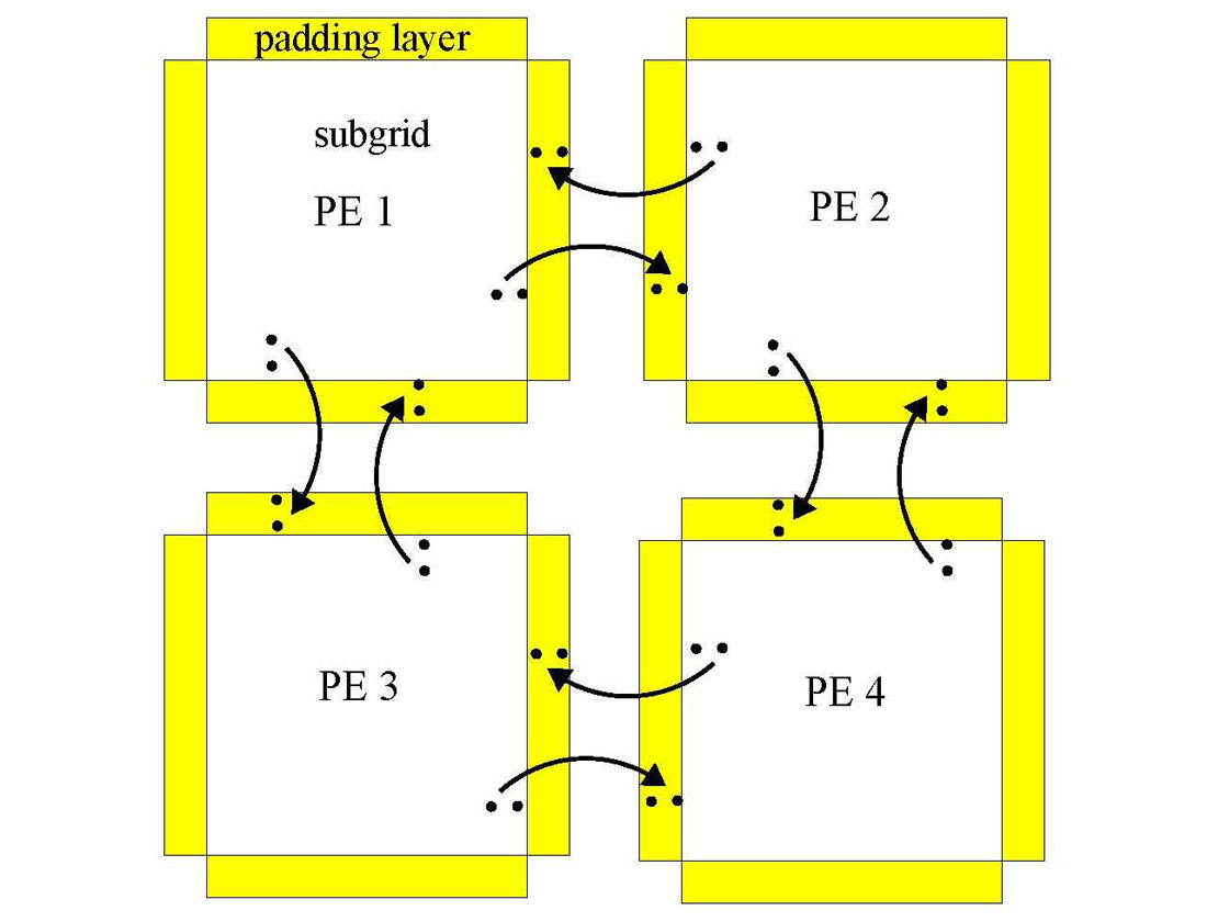
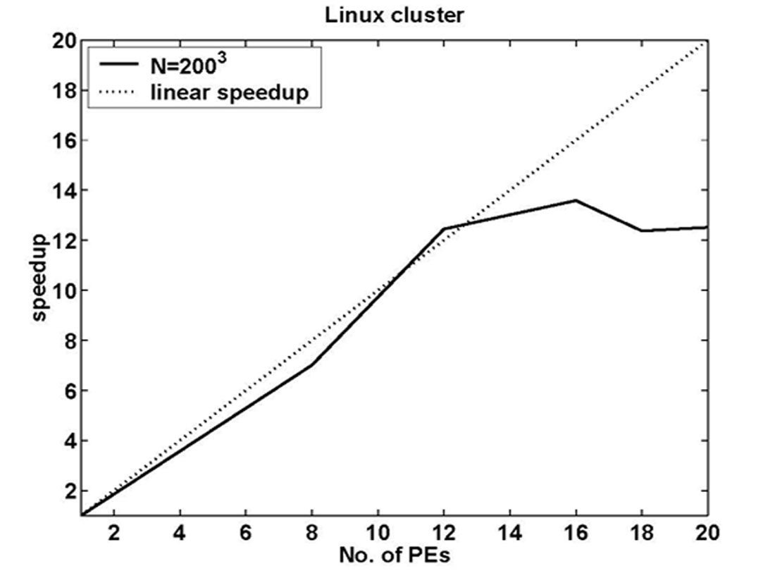
A large-scale model can be decomposed into sub-models which are assigned to each processor (Figure 1). Wavefield information is exchanged among internal processors while processors at the edges will provide pre-defined boundary conditions. Communication thus plays an important role in reducing calculation time. A trade off can be observed between speedup and number of processors (Figure 2). Due to high communication times for large PC numbers, performance does not improve for PC numbers above a certain threshold.
P- and S-wave Energy Separation
The computation of the total elastic wave field allows the separation of P- and S-wave energy through divergence and curl operations and display them in separated seismograms as well as conventional horizontal and vertical component seismograms. The displacement can be written as (Aki and Richard, 1980 Vol.1, P68)

where ∇φ and ∇xΨ are called P-wave and S-wave components of displacement. φ and Ψ contain P-wave energy and S-wave energy, respectively. Thus ∇.u=∇2φ and ∇xu=(∇xΨ) present P and S-wave components separately. In the 2-D case, the S-wave component with only one non-zero direction is scalar, while in 3-D cases, the shear component is a vector,

and Bohlen’s codes (2002) converts this vector to a scalar. The algorithm for P-wave and S-wave components is

Where EP and ES are the P- and S-component energy respectively, νi denotes particle velocity in the i direction, π = λ + 2μ and μ are the compressional modulus and shear modulus of the viscoelastic media, respectively.
Strong Contrasts and Scattering
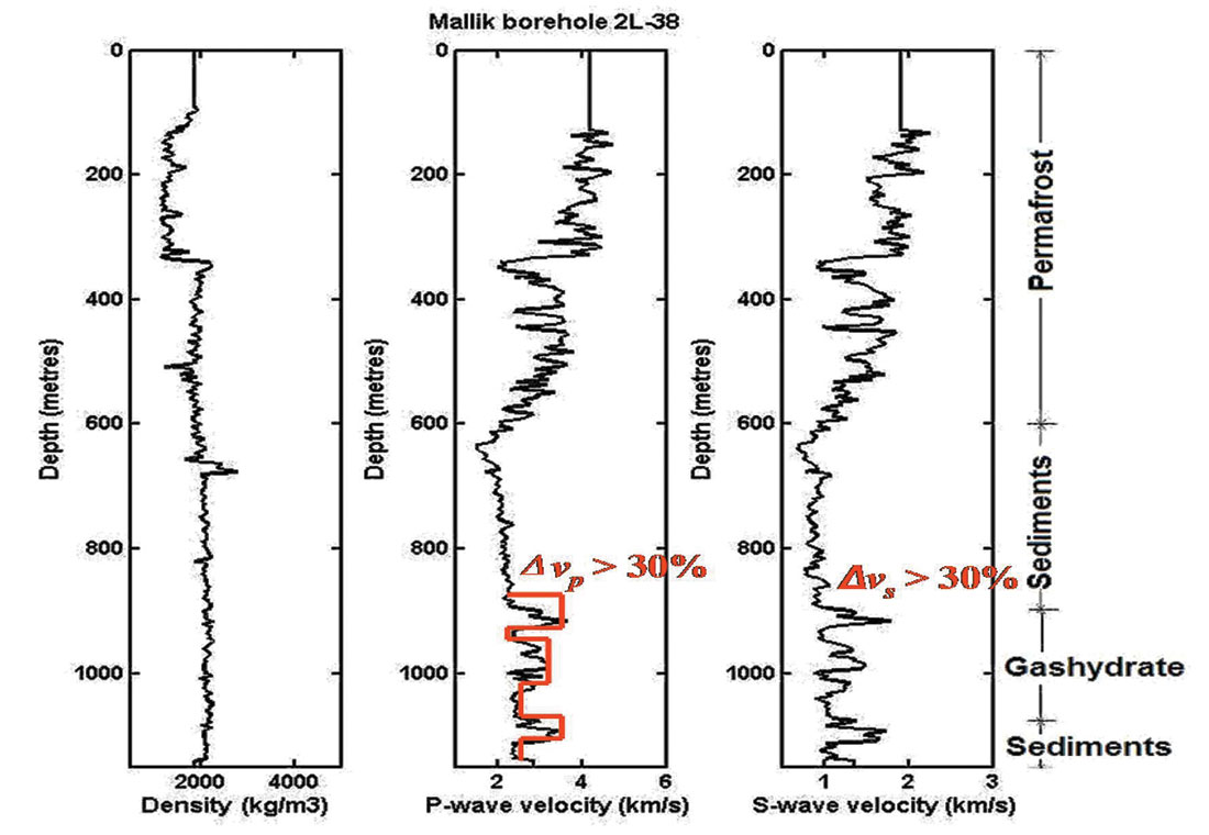
The accumulation of gas hydrates elevates both compressional and shear velocities (Milkereit et al. 2005) by over 30% and thus forms strong contrasts in non-gas-hydrate-bearing sediments. Strong negative P-wave contrasts are associated with over-pressured free gas pockets within near surface sediments are a potential hazard to drilling. Its presence is characterized by strong contrasts of both velocities and densities. Examples of strong contrasts are listed in Table 1. We chose gas hydrates accumulated in soft, water-saturated sediments as a simple case to simulate seismic scattering due to strong contrasts and limited lateral scales of P-wave velocity. Viscoelastic influence is applied to the heterogeneous model by assigning a constant Q value to the model.
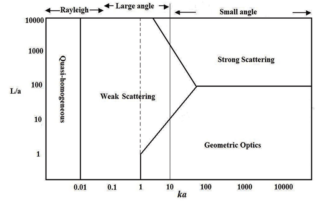
Wu (1989) classified four scattering regimes (Figure 3) based on the wavenumber of seismic waves (k) and the scale of heterogeneities (a): quasi-homogeneous (ka<0.01), Rayleigh scattering (ka<<1) , large angle scattering (0.1<ka<10), and small angle scattering (ka>>1). Seismic wave behavior is thus frequency and scales dependent.
| Free gas in porous sediments | Gashydrates reservoirs | |
|---|---|---|
| Table 1. Strong scattering examples for gas reservoirs. λ is the range of seismic wave length for frequencies around 30 Hz. Gas hydrate reservoirs show both compressional and shear velocity contrasts while free gas only has compressional velocity contrast. Δυ=(υscatter -υbackground)/υbackground, Δd= (dscatter-dbackground) /dbackground, (from Müller 2000, p26, and Milkereit et al., 2005). | ||
| Δυp | 0 | 45.5% |
| Δd | 0 | 0 |
| υp/νs | 2.0 | 2.0 |
| λ(m) | 100~500 | 100~400 |
Case Study Results
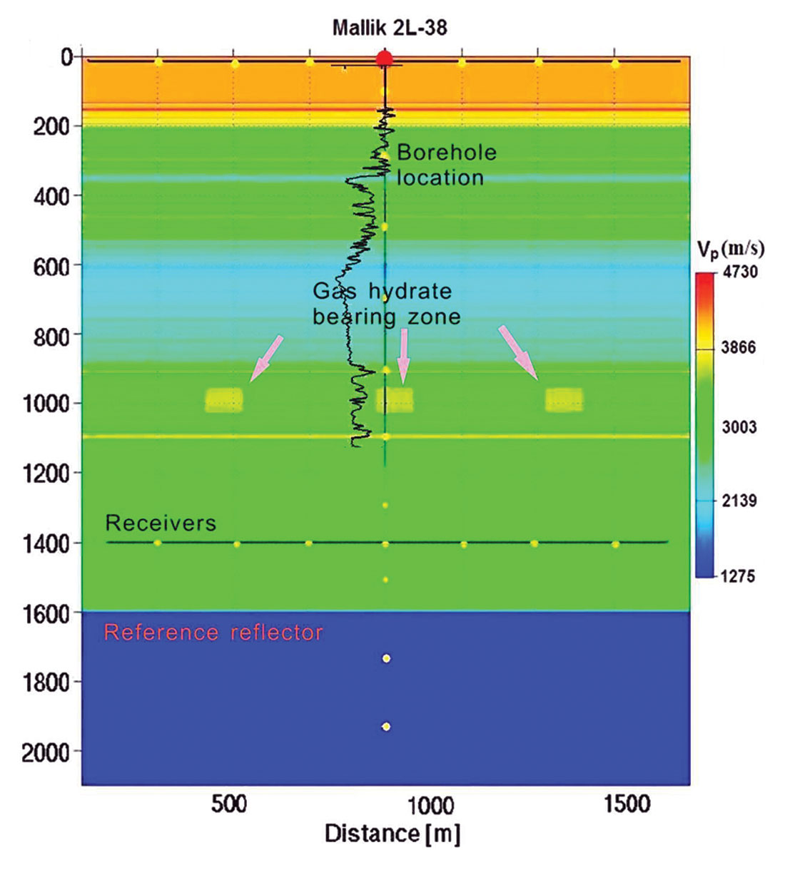
A seismic survey and research wells from the Mackenzie Delta, Northwest Territories of Canada provide complete field data including well logs, seismic data, and geological information ( Dallimore and Collett, 2005). To construct an unstratified model, a 2-D patchy model based on logs from Mallik 2L-38 (Figure 4) was constructed with acquisition geometries shown in Figure 5. The patches are 100 m wide at a depth between 950 m and 1030 m.
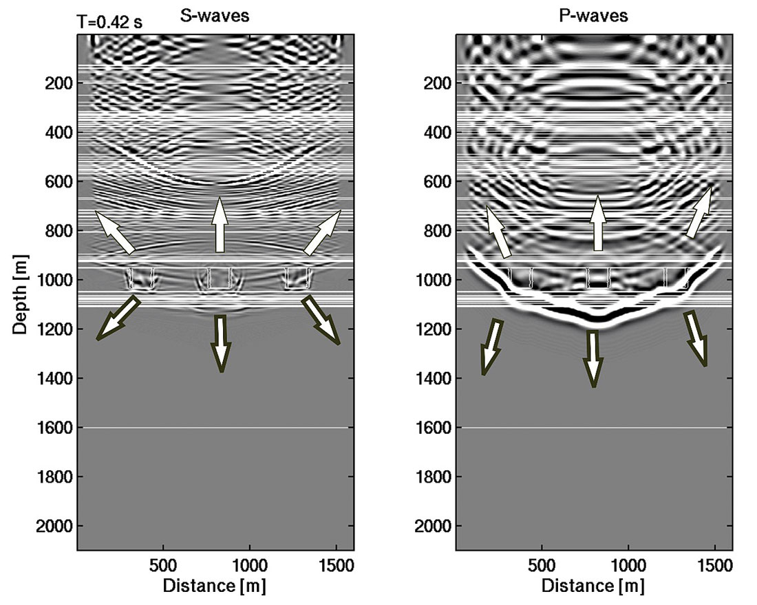
Two sets of elastic wave fields are generated by an explosive source and a compressional plane wave, respectively. The total synthetic wave field, including reflection, transmission, and Vertical Seismic Profile (VSP) data, are recorded for analysis. The wave front distortion, weak backward scattering, and strong P-to-S conversion due to lateral discontinuity of impedance are visualized in the snapshots of both wavefields (Figure 6) at the same time. The directions of scattered waves are consistent with the theoretical prediction (Wu, 1989). The role of composition and shape of scatters was analyzed in the elastic seismic-wave scattering from massive sulfide orebodies (Bohlen et al., 2003).
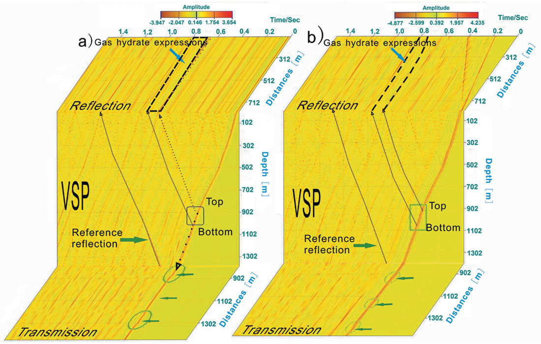
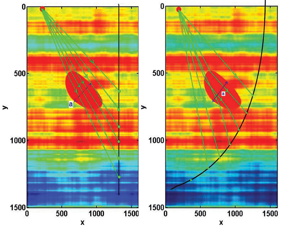
The combination of synthetic reflection, VSP, and transmission data provides another way of visualizing and analyzing the seismic data (Figure 7). Synthetic seismograms as follows are display with Seismic Un*x (Forel et al., 2005). Seismic expressions of patchy structures can be traced with ease from synthetic zero-offset VSP data to the two-way-travel time (TWT) reflection data. The amplitude variations in synthetic transmission data indicate that scale information may be easier to extract from transmitted energy than from reflections. Walk-away VSP and VSP conducted in deviated boreholes (Figure 8) are favored acquisition geometries to extract scale information from transmitted energy. Forward modeling can be of assistance to designed and evaluate seismic 3-D VSP acquisition geometries.
Conclusion
Parallel 3-D Finite Difference modeling (FD) codes provides a powerful tool to simulate seismic wave propagation in complex geological settings including strong contrasts, small scale heterogeneities, viscosity, etc. They can be quite accurate, if methods to reduce numerical dispersion are applied. FD was applied to simulate seismic scattering due to lateral variations of physical properties, e.g., patchy gas hydrate distribution. In addition, 3-D forward modeling studies may aid 3-D seismic survey design and data interpretation.


Join the Conversation
Interested in starting, or contributing to a conversation about an article or issue of the RECORDER? Join our CSEG LinkedIn Group.
Share This Article