Non-first-break technology to remove effects of shallow velocity anomalies

As was analytically shown in the first paper (Blias, 2006a) shallow velocity anomalies can cause large lateral variations in stacking velocities. Non-removed shallow velocity anomalies (SVAs) can reduce the quality of the post-stack image and create time distortions in seismic horizons. A conventional approach to deal with SVAs utilizes first breaks to determine shallow velocity structures (Hampson and Russell, 1984, Yilmaz, 1987, Cox, 1999). In some cases the first break approach does not work because of poor first break determination, a shallow low velocity layer, or permafrost among other possible problems. In these cases we can sometimes use reflections to restore SVAs and to remove their effects on seismic data.

There are three main approaches to build depth velocity model:

1. Direct inversion of NMO velocities and zero-offset times: Dix type of method, including generalizations of Dix formula
2. Different types of reflection tomography.
3. Prestack depth migration velocity analysis.

The first type of approach (direct inversion) works on a layers-tripping method except for a 1D model when the Dix formula gives the solution using only two reflections – at the top and at the bottom of the layer. If we estimate an interval velocity for 2D and 3D models (that is when the 1D local assumption does not work) we have to know the velocity distribution in the overburden. In the presence of unresolved (that is with unknown shallow anomalies) shallow velocity anomalies, any kind of direct inversion will lead to big errors because the difference between NMO velocities for the model with and without shallow velocity anomalies is big (it’s increasing with reflector depth).

The second and third type of approach (any kind of reflection tomography, prestack depth migration velocity analysis) requires a reasonable initial approximate velocity model. To find an initial model, we can try to use Dix type of inversion, which does not require initial model, but in the presence of unresolved shallow anomalies, it will not give reasonable interval velocities. That is why, before using any reflection tomography or prestack depth migration velocity analysis or ray-based stacking velocity inversion, we need to develop a method to obtain appropriate initial depth velocity model including the shallow part of the subsurface. After that we can use reflection tomography approach to improve this model. We can say that tomography and prestack depth migration approaches were developed for the situation when the shallow part of the subsurface is simple and complex structures are relatively deep. In this paper, I consider the opposite case – shallow velocity distribution is complicated (shallow velocity anomalies) and we don’t have shallow reflection, but deep geology is gentle.

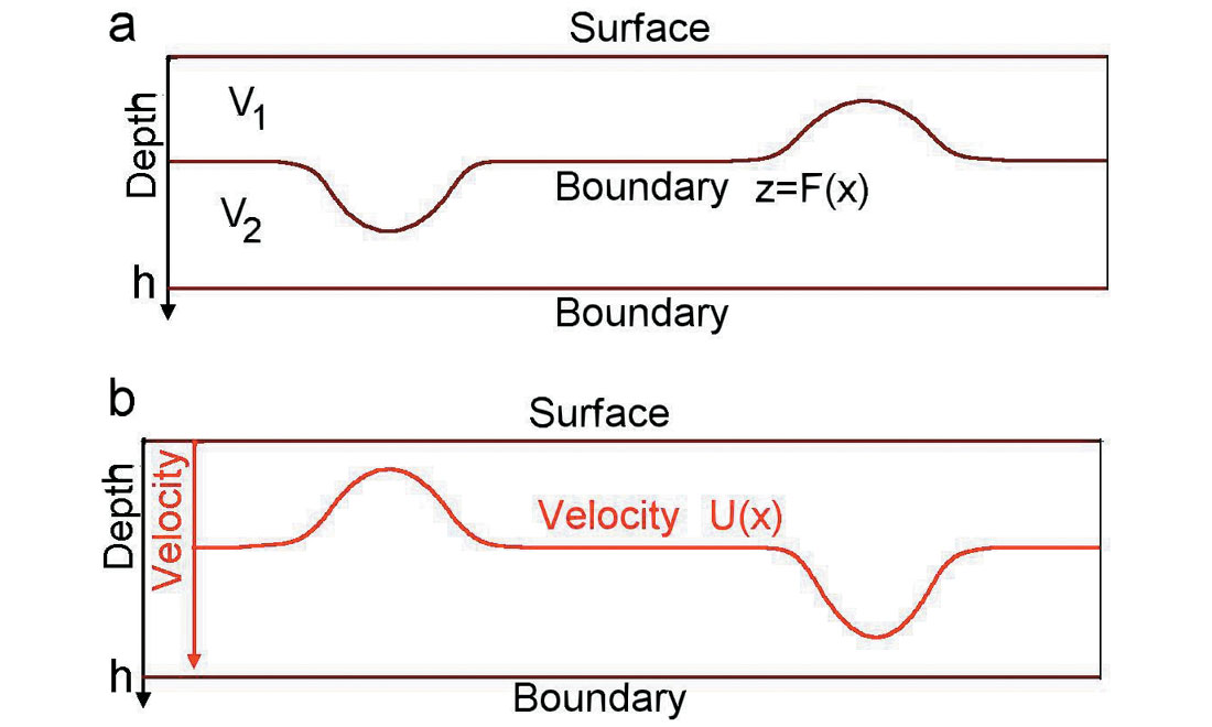
There are two possibilities to describe shallow velocity anomalies. We can use a curvilinear boundary z = F(x), which separates two layers with constant velocities, fig. 1a. We may also use a laterally inhomogeneous layer with the velocity u(x), fig. 1b. Let’s assume that the interval velocity in the second model gives the same vertical time in the first layer as in the first model within the layer between 0 and the depth h. It means that we have a connection between the boundary F(x) and velocity u(x) (Fig. 1):

where s(x) is slowness in the layer: s(x)= 1/u(x). After differentiating this equation twice, we come to the connection between the second-order derivatives of the two forms:

Comparing formulas (1) and (2) from the paper (Blias, 2006a) and taking into account the last formula, we see that both shallow velocity anomaly descriptions give close to NMO velocities. It means that if we describe a shallow velocity anomaly using either a laterally changing interval velocity or a curvilinear boundary, we will come very close to the same result.

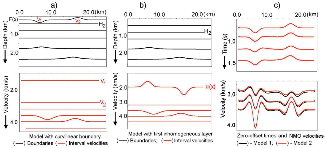
To illustrate this, let’s consider two models with shallow velocity anomalies, as shown in Figure 2. In this example, we use the two descriptions of the shallow velocity anomalies. Both models have two shallow velocity anomalies. For the first model, these anomalies are described with a curvilinear boundary F(x) as Figure 2a. The second model, with a laterally changing interval velocity in the first layer, is shown in Figure 2b. Both descriptions give the same vertical time in the first layer, that is, equation (3) holds. Figure 2c shows NMO parameters for these two models. We see that the NMO parameters for these two models are almost the same. It means that we can use either of the descriptions to build a shallow velocity model from time arrivals. Which one to use depends on a priori information about shallow velocities.

Technology for non-first-breaks removal of shallow velocity anomaly effects

Based on these results, a special technology has been developed (Blias, 2005a,b). Most of the coding has been developed by Valentina Khatchatrian. This technology includes five main steps.

1. Automatic high-density non-hyperbolic constrained velocity analysis. To run this velocity analysis, we first pick velocities at one CDP gather and put some constraints on how rapidly these velocities can change laterally and on the possible values of stacking velocities (Blias, 2006b). The result of this step is a velocity section for each CDP point and each time sample. NMO gathers are considered as a QC for the velocity analysis result.
2. Building initial depth velocity model. For this we use the stacking velocities after the first hyperbolic velocity analysis. First we determine the shallow velocity model using deep reflections (Blias, 2005b). After that we use a generalization of the Dix formula for a layered medium with laterally varying velocities (Blias, 2003a)
3. Travel-time inversion and depth velocity model improvement. We use non-hyperbolic travel-times to build a depth velocity model, including shallow velocity structures. For this we use a layer based optimization approach (Blias and Khatchatrian, 2003b). We describe interval velocities and boundaries as the sum of some reference (known) functions and linear combinations of basic functions jk(x,y) with the coefficients a and b:

   

   
   Here ϕ_k(x,y) – basic functions, α_m,_k, β_m,_k are unknown coefficients for the m-th layer; ρ_m(x,y) and H_k(x,y) are slowness and boundaries for the zero approximation of depth velocity model (reference model). Then we can calculate the objective function

   

   
   Here k is the number of reflections that are used; t_k(S,M) is observed time for the k-th wave, S and R stand for the source and receiver points. Scalars u_m and w_m are regularization factors to stabilize the solution of the inverse problem. To find a minimum of the non-linear function F, we use the Newton method.
4. Velocity anomaly replacement (VAR). We use the depth velocity model to remove the influence of the SVA. For a given shallow velocity model it can be done by forward and reverse prestack wavefield extrapolation (Wapenaar and Berkhout, 1985). We use variable time shifts to remove SVA effects, which is much less expensive (Blias et al, 1985). For this we run raytracing for the obtained depth velocity model and calculate prestack reflection time arrivals for all boundaries. Then we replace the shallow inhomogeneous layer with a homogeneous one and calculate time arrivals for this model. The difference between the first and the second set of times is applied to CDP gathers. This procedure moves events on prestack data to the position where they would be if the shallow layer were homogeneous.

Model data test

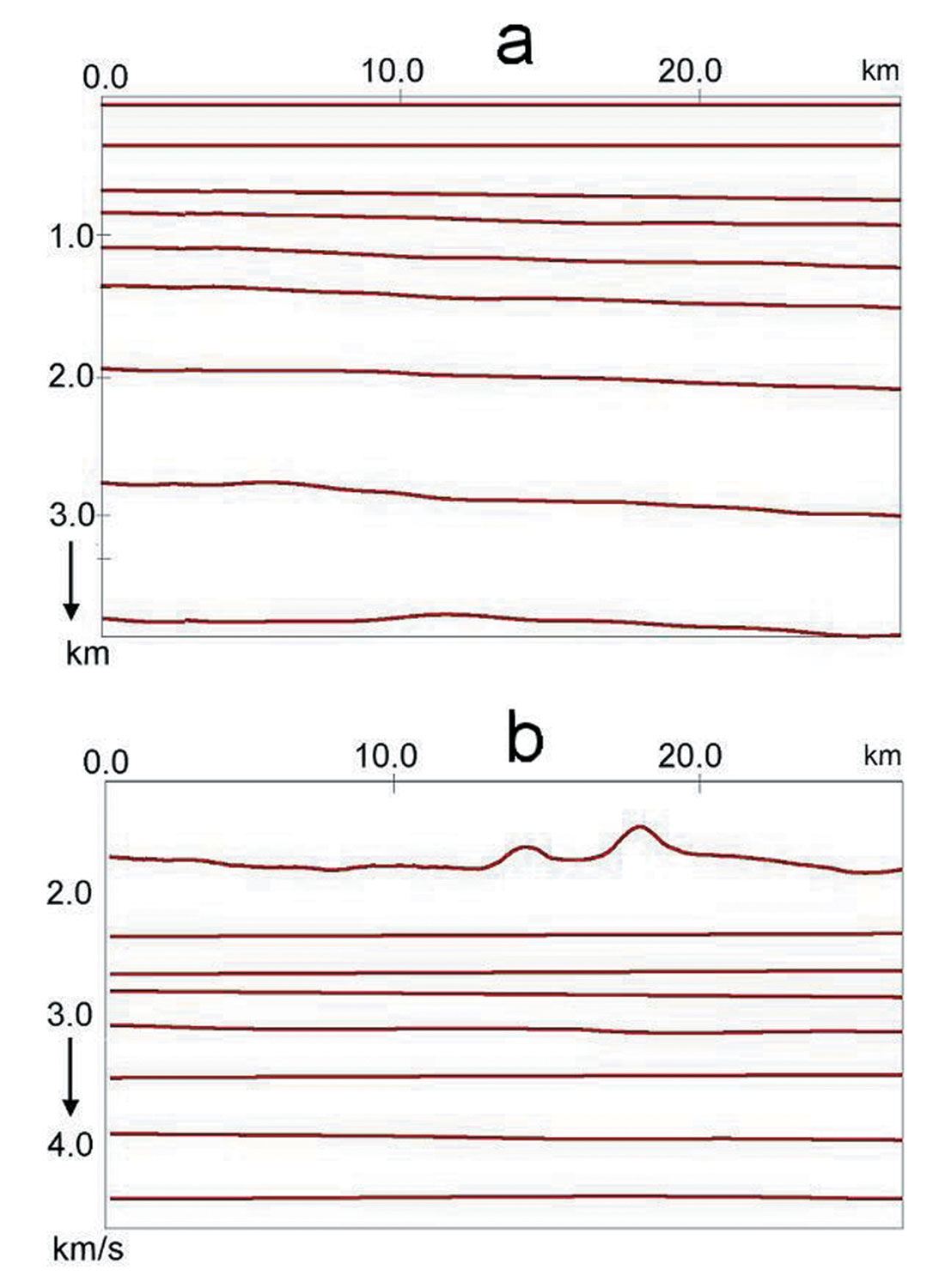
Let’s illustrate the above technique on model data. We test this approach on model data with modest deep structures. We will see that the suggested approach is stable and allows us to restore the depth velocity model when we have complicated shallow velocity anomalies, caused by several curvilinear boundaries and laterally inhomogeneous layers. Figure 3a shows depth velocity model boundaries and interval velocities are displayed on figure 3b.

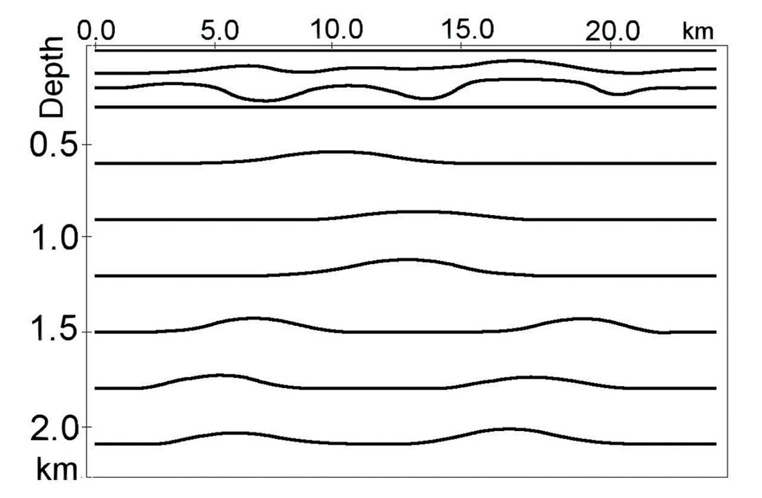
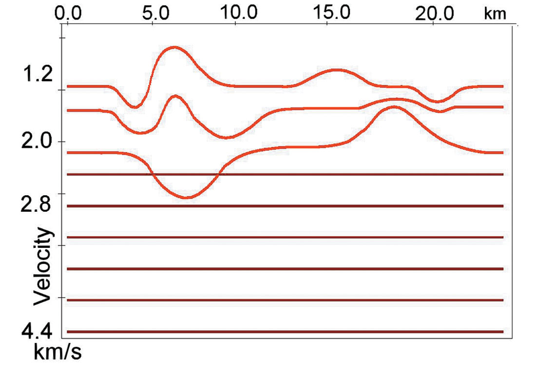
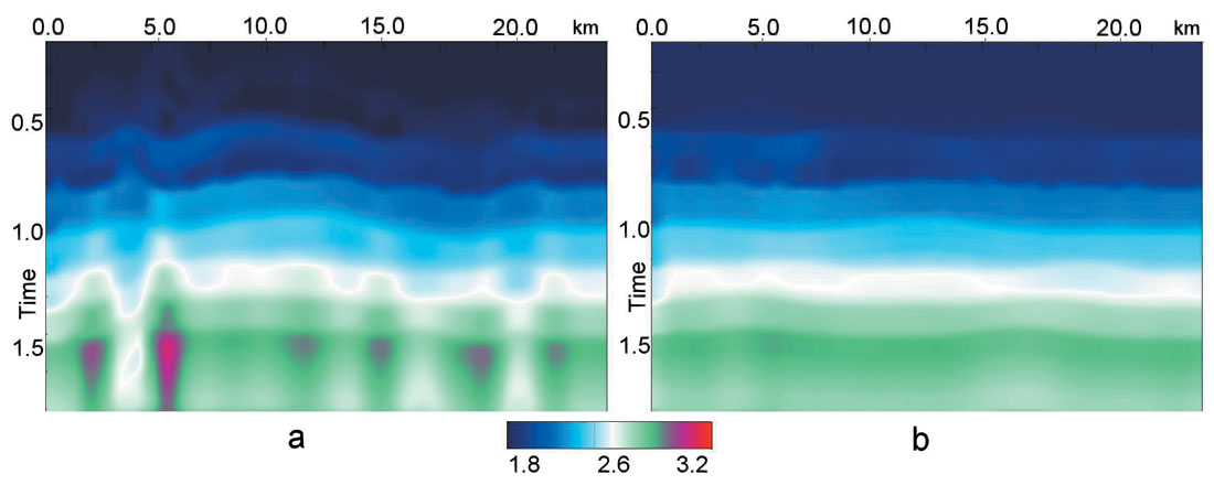
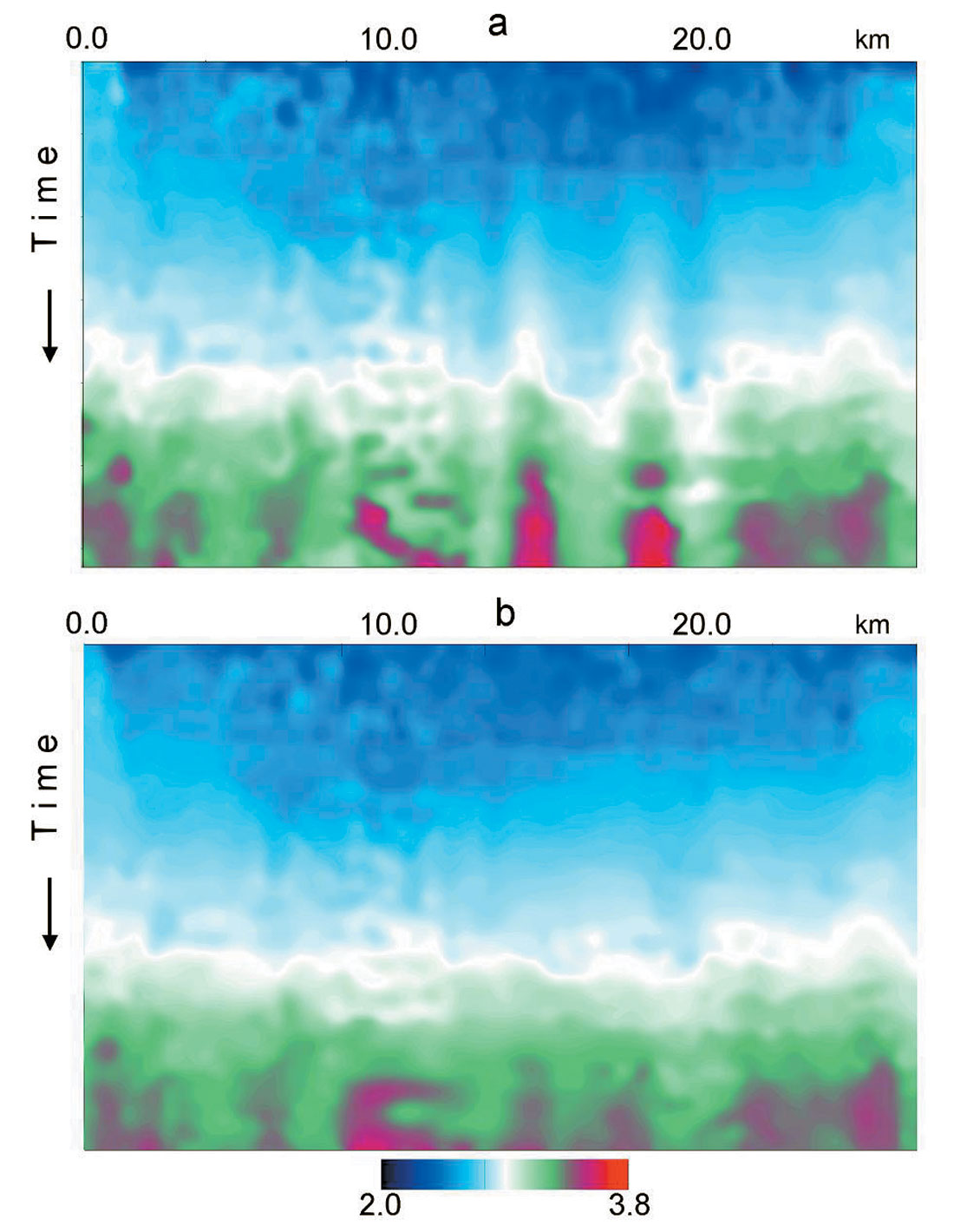
From these figures we see that the shallow part of the subsurface is complicated. The bottom of this shallow part is set to 300m. Above this boundary there are three curvilinear layers with laterally changing interval velocities. The average velocity in this layer is 1600 m/s. For this model synthetic CDP gathers have been calculated with maximum offset/ reflector depth = 1.5. Shot interval = receiver interval = 32 m. All 5 steps have been run on this synthetic data. Figure 4a shows a velocity grid after automatic continuous velocity analysis. We see large lateral stacking velocity oscillations increasing with depth.

An initial velocity model was build, using the methods from the author’s papers (Blias, 2003, 2005). To build the initial depth velocity model we need to assign an average velocity in the first layer. We put h₁ = 240m and average velocity in the first layer of 1200m/s while we know that h1 is 300m and average velocity in this layer is 1600 m/s. It means that we have used the wrong a priori parameters for the first layer to prove that it should not have much influence on the final result of shallow velocity anomaly replacement.

To improve this model, traveltime optimization inversion was applied using non-hyperbolic traveltimes extracted after residual velocity analysis.

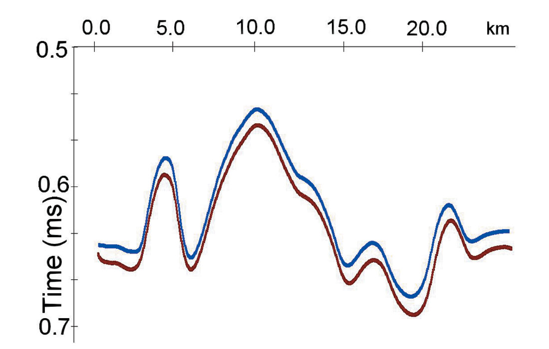
Because we used the incorrect value for the bottom of the first layer with velocity anomalies (240 m instead of 300 m) the recovered velocity in this layer differs from the original average velocity. As was mentioned above, the vertical time should be found with a reasonable accuracy. Figure 5 shows vertical times for the original model (blue) and for the model after traveltime inversion (brown).

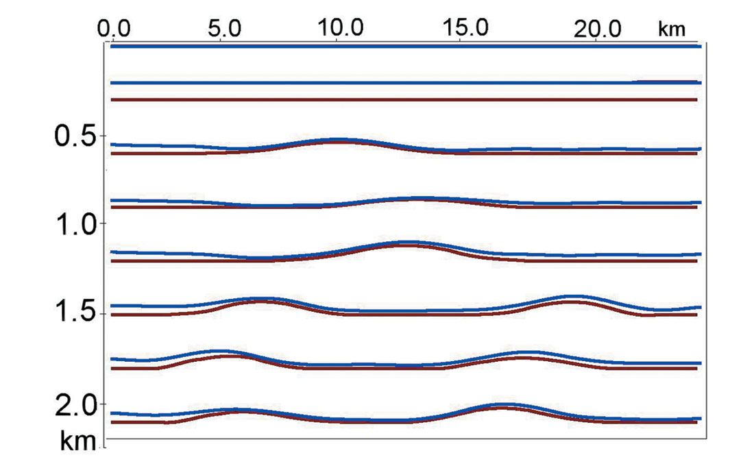
After we determined the interval velocity in the first layer, we use a generalization of Dix’s formulas (Blias, 2003) to find interval velocities for the other layers. The results of these calculations give us the initial depth velocity model, which is needed for the optimization traveltime inversion. Figure 6 shows the boundaries of the initial model (brown) and after optimization (blue). Comparing these with the original model boundaries (fig. 3a) we see acceptable similarity between them. All structures were recovered correctly despite using the wrong thickness for the first layer.

The model after traveltime inversion was used to calculate VR corrections. These corrections were applied to CDP gathers. They transform moveout curves to hyperbolic ones (strictly speaking, new NMO curves can be better approximated with a hyperbola than the original ones). VR significantly removed non-hyperbolic distortions caused by shallow anomalies.

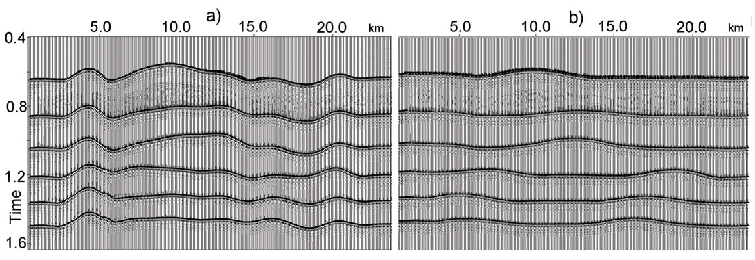
VR also significantly improved the velocity grid (fig. 4 b) and structural imaging. Figure 7 shows poststack sections before (a) and after (b) VR. We can see that after the VR the poststack data looks more similar to the depth velocity model. From this we come to conclusion that, for the shallow part of the section, utilization of a laterally inhomogeneous layer instead of complicated velocity model is acceptable. It allows us to restore shallow velocity anomalies using deep reflections and to eliminate their influence on prestack gathers with sufficient accuracy.

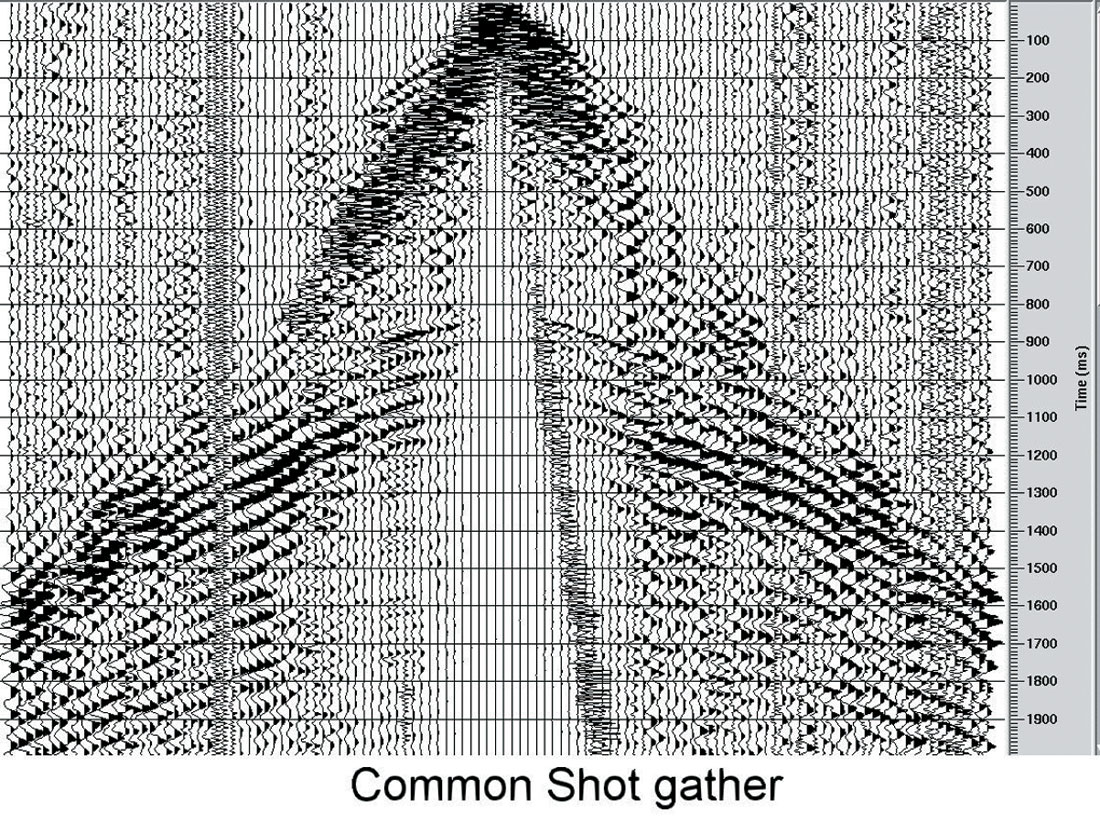
Real data example. The quality of raw data did not allow us to use first breaks at all, so the only information that we could use was reflection traveltimes (Fig. 8).

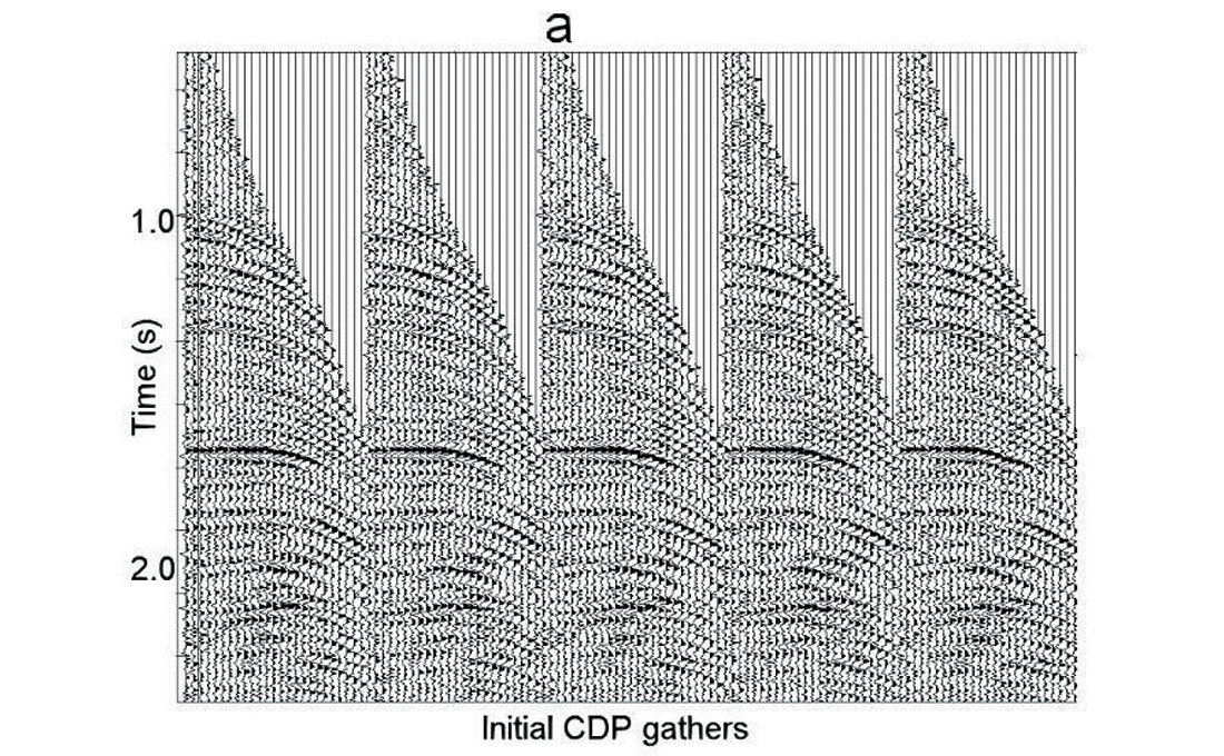
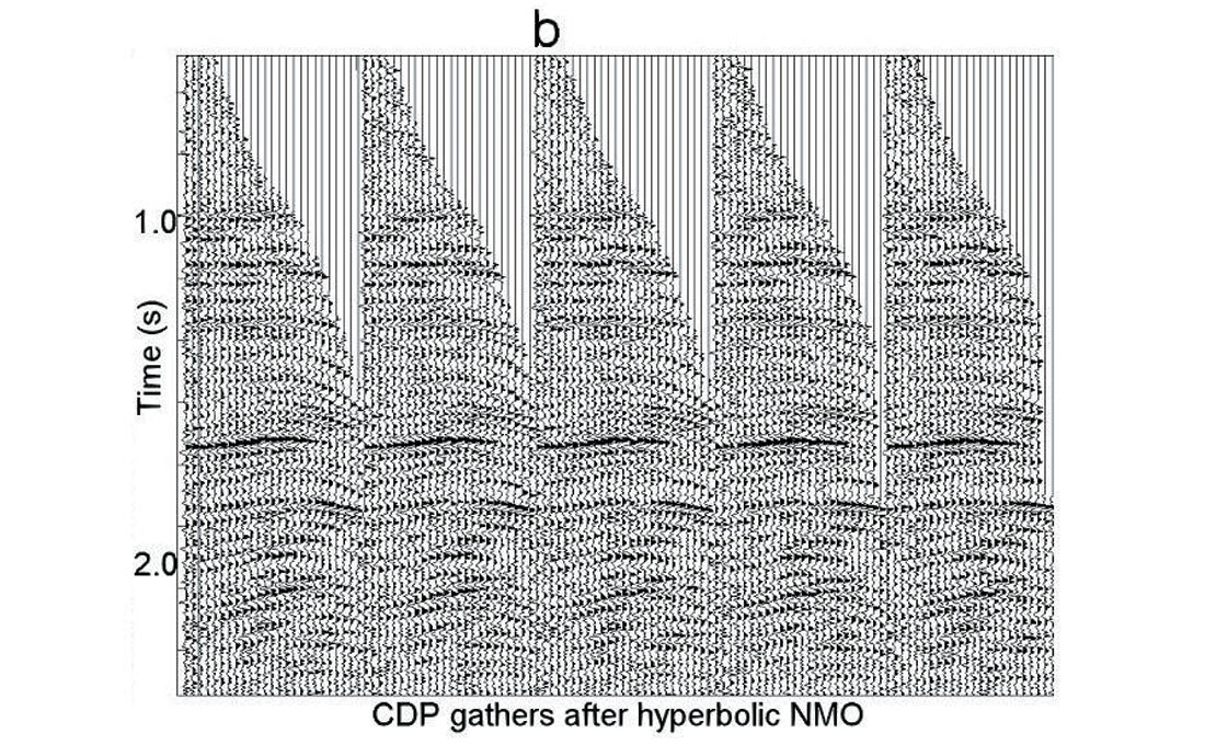
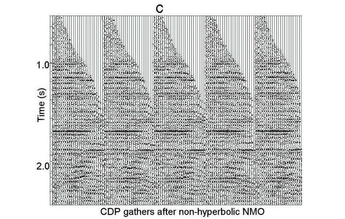
After automatic high-density non-hyperbolic velocity analysis we determined NMO curves with high accuracy. Figure 9 shows initial CDP gathers (a), NMO gathers after hyperbolic velocity analysis (b) and after non-hyperbolic residual velocity analysis (c). We see strong non-hyperbolic NMO and flattened arrivals after automatic non-hyperbolic velocity analysis.

Picked traveltimes were used to build a depth velocity model using a generalization of Dix’s formulas and optimization approach. The result is shown in figure 10. We see a strong shallow velocity anomaly in the interval 12 – 18 km.

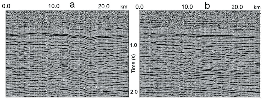
After depth velocity model building, we replaced the shallow velocity. For improved CDP gathers, the continuous automatic constrained velocity analysis has been applied (Blias, 2006b). Because of shallow velocity anomaly replacement, stacking velocities do not have specific variations caused by shallow inhomogeneity (Fig. 11). Figure 12 shows seismic sections before (a) and after (b) shallow velocity anomaly replacement. We can see significant changes in the interval between 15 and 22 km. Velocity replacement eliminated horizon fluctuation within this interval and improved the stacking velocities.

Acknowledgements

We would like to thank Michael Burianyk (Shell Canada) and Jason Noble (Edge Technology) for helping me with this paper. I would like to acknowledge Valentina Khatchatrian who developed most of the software and Samvel Khatchatrian for useful discussion.