Noise Examples from Two Microseismic Datasets

Abstract

The recording of microseismic surveys can be used to monitor hydraulic fracture stimulation of reservoirs. In these surveys, the continuous recording of three component geophones are used to detect P and S wave energy induced by the fracturing process and related stress changes. This paper presents a number of noise examples recorded on two microseismic datasets from Canada. The noise can be high in amplitude, persistent in time, and may adversely affect the recording of P and S wave signal energy.

Introduction

Microseismic methods have emerged as an important tool for hydraulic fracture monitoring (HFM). The purpose of recording microseismic data is to locate individual fractures and fracture networks introduced into a reservoir. The microseismic data are recorded at high sampling rates over the duration of the fracture stimulation. Three component geophones are usually used to record the data. The geophones may be placed down an observation well and clamped to the side of the borehole casing. This may allow for recording significantly higher frequencies than those recorded at the surface.

Along with the signals of interest (i.e. P- and S-waves produced by the microseismic events), various types of noise (random or coherent) may be recorded during a microseismic survey. For the purpose of this paper, noise is defined as anything other than P and S wave energy. Examples include electrical noise from the recording equipment or waves that propagate within the borehole casing. Noise can also be generated by the geometry of a downhole geophone array. The examples shown here are the results of the analysis of hours of microseismic data. The examples are typical of many events that have been recorded.

Signal Example

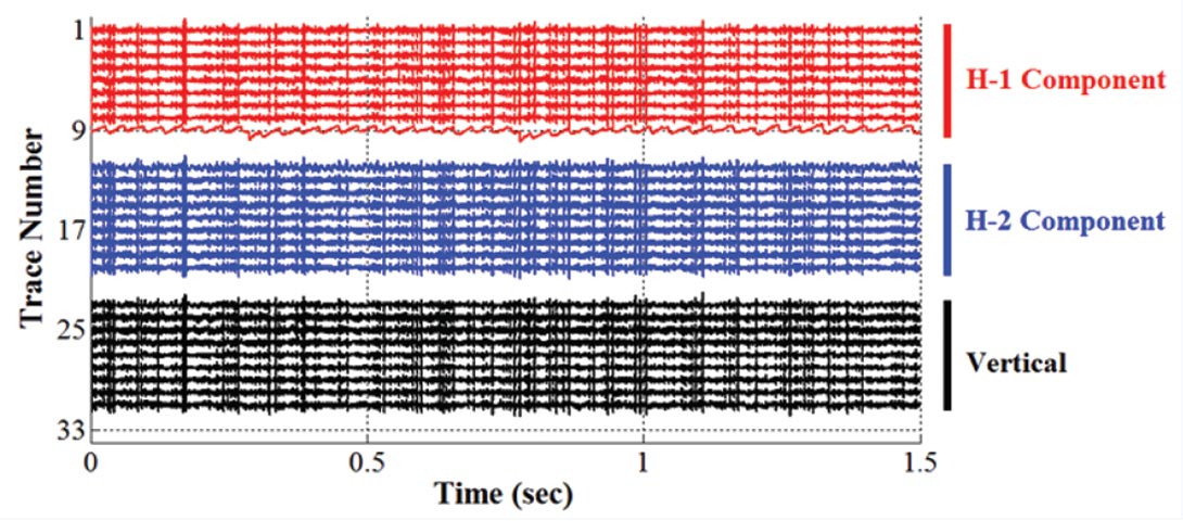
Before the noise examples are presented, a typical signal example is shown for reference. Figure 1 is one 1.5-second window from a six-hour recording of a multifrac treatment that was performed in Alberta in the winter of 2010. Twelve three component geophones were recorded in a vertical observation well about 600 meters away from the horizontal treatment well. The deepest geophone was about 60 meters from the bottom of the observation well (just above the fractured zone); the other geophones were spaced at 30 m shallower intervals. At about 0.7 seconds, there is a P wave arrival that is followed by a stronger amplitude S wave arrival. This is typical of primary signal evident in the three datasets analyzed in this study. The P wave energy is low in amplitude compared to the S wave energy. The traces here are raw unfiltered data.

Random Noise

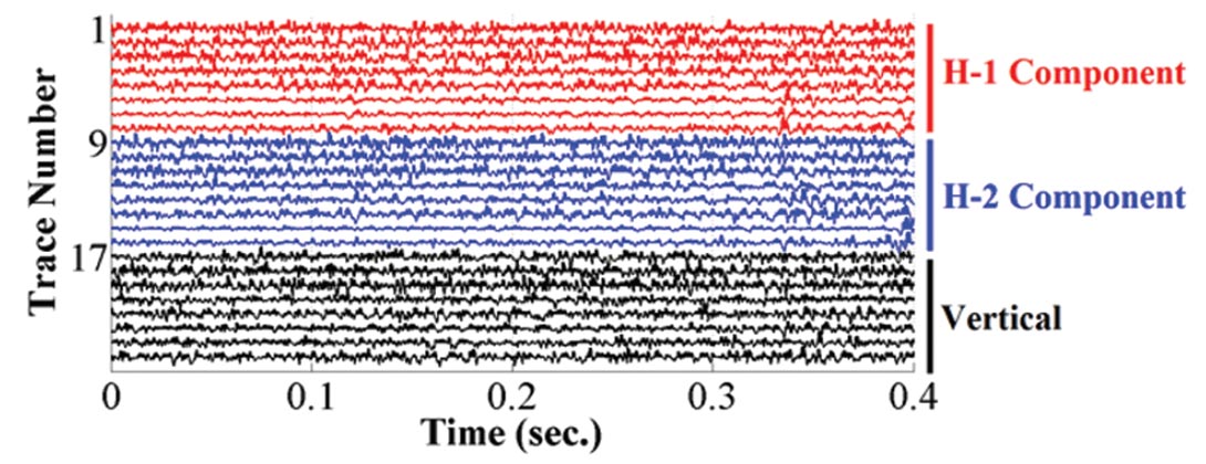
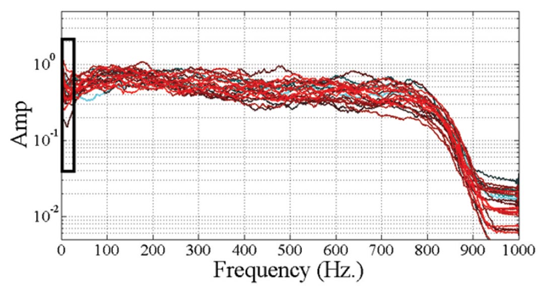
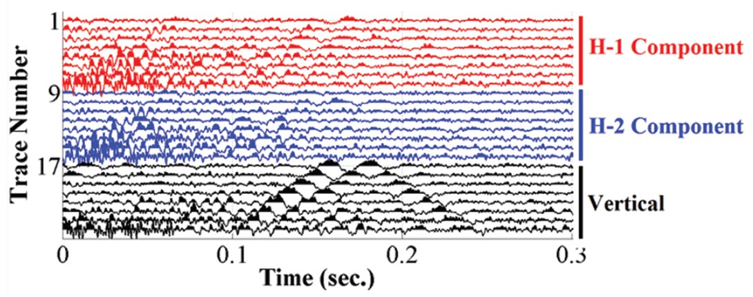
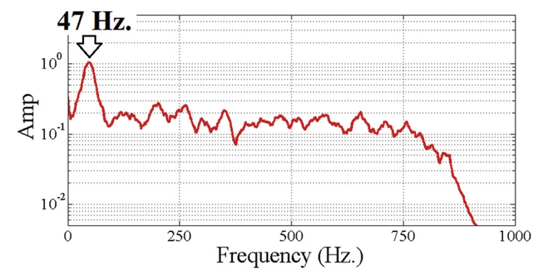
Figure 2 is a 0.4 second window from a second Alberta survey. The traces appear to be uniform random noise similar to surface seismic random noise. However, consider Figure 3. The broad spectrum of the noise ranges from D.C. to about 800 Hz., at which point it drops to the 1000 Hz. Nyquist frequency. Figure 3 shows that some of the traces have a D.C. component. This component can hurt programs such as autopicking algorithms or deconvolution.

Noise Example: Almost “Dead” Trace

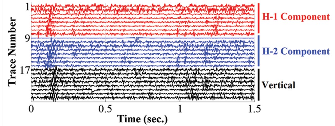
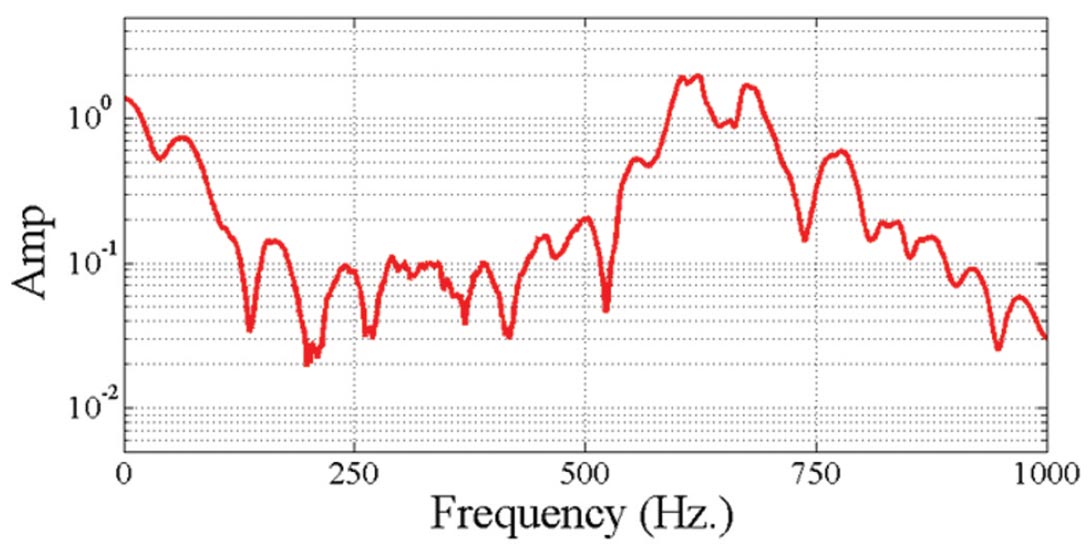
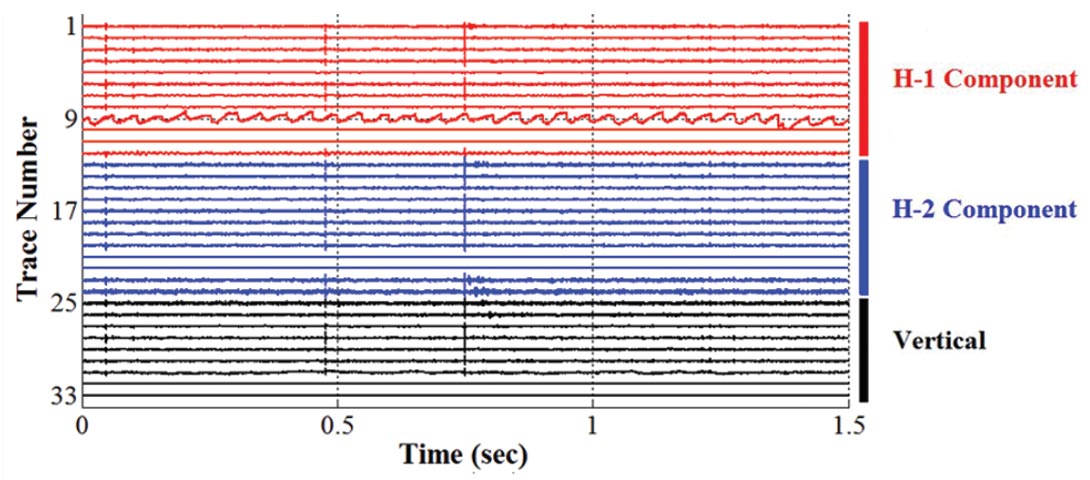
Figure 4 is another 1.5 second window from the second Alberta dataset. There is a S wave arrival at about 0.15 seconds on most of the traces, except trace 9. This shallowest H-2 component geophone has recorded a noise spike. The cause for this recording is currently unknown and may warrant further investigation. Figure 5 shows the frequency amplitude spectrum for this trace. Again, this noise trace contains a D.C. component that would affect autopicking algorithms or velocity semblance routines.

Electrical Noise and a Poorly Clamped Geophone

Figure 6 is a 1.5 sec. window from a hydraulic fracture that was performed in northeast British Columbia in the winter of 2010. Electrical noise is recorded numerous times on all channels except trace 9, which is the deepest H-1 geophone. It appears that this geophone may be poorly clamped and vibrating against the casing at about 28 Hz. This noise was observed in six minutes of data.

Tuned Response of a Clamped Geophone Array

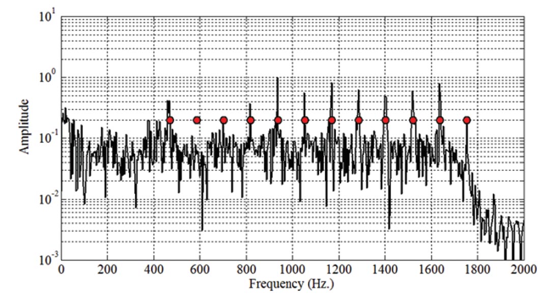
Figure 7 is 1.5 second recording from the same dataset that is shown in Figure 6. The vertically aligned electrical noise has subsided. Figure 8 shows the frequency amplitude spectrum for trace 29 from Figure 7. This trace appears to contain random noise and a few electrical spikes. The frequency amplitude spectra is not representative of uniform random noise; there are frequency spikes that begin at 467 Hz and at intervals of 117 Hz thereafter.

The frequency spikes in Figure 8 are caused by the clamped geophones in the wellbore acting as longitudinal stiffeners within the steel casing. This wellbore used Type 40 casing steel, which has a P wave velocity of about VP = 5,778 m/sec. The contractor recorded the spacing between each clamped geophone to be 12.37 m. The resonant frequency of a steel tube with stiffeners X meters apart is given by:

Also, there would be local maxima (mode resonances) generated above this fundamental frequency given by:

Equation 2 predicts that the clamped geophones are predicted to create nodal maxima at:

These predicted maxima are shown as red dots in Figure 8. The peaks starting at 467 Hz and incrementing by 117 Hz correspond to the predicted values for the system within 1 Hz. This phenomenon continues to be investigated by the Microseismic Industry Consortium.

Tube Wave (Stoneley Wave)

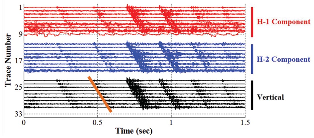
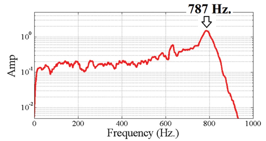
Figure 9 is one 1.5 second window from the Alberta dataset shown in Figure 1. There are six linear events that are high very amplitude and appear on all 24 channels. A straight line through the first arrivals of the energy gives an apparent velocity of 1460 m/sec. Figure 10 shows a peak frequency for trace 18 from Figure 9 to be about 787 Hz. By analogy with other studies (eg. Le et al, 1994), this noise train is thought to be a tube wave propagating the borehole. This noise is similar to that predicted by Rama Rao and Vandiver (1999) as a “Mode 2” Stoneley wave propagating between the steel casing and the casing cement. The source of the tube wave is from the top of the geophone assembly – it may have been a P or an S that was converted to a Stoneley wave or it may have been induced at the surface. The tube waves are high amplitude and affect all geophones; they may obscure the arrival of P wave or S wave signals.

P Wave in the Casing Cement

Figure 11 shows two high amplitude linear events from the Alberta dataset. There are very high amplitude events on the vertical component, but only a few horizontal traces record any of this motion. A straight line through the first arrivals of the vertical component energy gives an apparent velocity of 4,200 m/sec travelling down the borehole. This velocity is approximately equal to the P wave velocity for in the casing cement (Tang and Chang, 2004). The later event on the vertical component also has an apparent velocity of about 4,200 m/sec, but travelling down the borehole. This down-going wave may be the result of a reflection of the upgoing wave from an impedance contrast.

Figure 12 shows a peak frequency for trace 18 from Figure 9 to be about 47 Hz. This implies a dominant wavelength of about 89 meters. The P wave in the wellbore cement is high amplitude and affects all vertical geophones. This wave may obscure the arrival of P wave or S wave signals on the vertical geophones.

Conclusions and Future Work

A number of noise examples from the microseismic monitoring of two Canadian HFM surveys have been presented. The noise examples range from almost dead traces with no amplitude recorded to very high amplitude energy recorded on all traces. Characterizing sources of noise such as this is important for processing and interpreting microseismic data. The tuned response of the clamped geophone array introduces a frequency response that requires further investigation.

Acknowledgements

Sponsors of the Microseismic Industry Consortium are sincerely thanked for their support of this initiative.