Microseismic Geomechanics Interpretation of a Montney Hydraulic Fracture

In this paper, we describe the use of a geomechanical model to interpret microseismicity recorded during a Montney hydraulic fracture treatment. The microseismic geomechanical model is calibrated to the recorded microseismicity and used to understand the complete fracture network, including the proppant distribution. The calibrated model is then used to test different fracture and completion designs. The case study represents an example of enhancing the intrinsic microseismic value, by inferring engineering design improvements from existing microseismic data.

Introduction

Hydraulic fracture interpretation of microseismicity is typically focused on assessing the fracture geometry: specifically orientation, height, length and complexity often measured as the stimulated reservoir volume (SRV). Various engineering applications have evolved using microseismic to improve fracturing, completion and well designs (e.g. Maxwell, 2014). There are, however, apparently some cases with questions around value of information (VOI), where microseismic images identify the reservoir contact but do not lead to decisions around how to change operations. In contrast, the VOI is particularly clear in examples that involve comparing fracture systems resulting from different treatment or completions designs as a means to improve the design based on a preferred fracture geometry. However, microseismic applications of this type requires coordination of the monitoring project and operations to provide high quality microseismic data to assess different operations. Real-time monitoring can also be used to diagnose and correct unintended operational issues, such as screen-outs or completion issues. On-the-fly decisions of stage spacing are also a common approach to optimize the coverage along horizontal wells. Nevertheless, VOI from microseismic will come under increased scrutiny, particularly in the current economic conditions.

Microseismic interpretation has also evolved towards investigating rock deformation by characterizing the microseismic source strains, including methods such as moment tensor inversion. A growing number of published cases include characterizing an explicit microseismic fracture network and in some cases inferring the portion that contains proppant. However, rigorous interpretation of microseismic source characterization requires an understanding of the relationship between the microseismicity and the total geomechanical deformation. Microseismicity is often a shear dominated process corresponding to rock movements occurring with time frames consistent with seismic frequencies, and represents a small portion of the rock movement which is predominantly associated with the aseismic hydraulic fracture as a relatively slow and predominantly tensile process. Furthermore, microseismicity can occur from deformation directly associated with the pressurized, hydraulic fracture fluid flow (so called ‘wet’ events) but also remote from the hydraulic fracture as a result of stress changes (‘dry’ events). Therefore, to confidently interpret microseismic sources, a geomechanical framework is required which examines conditions leading to both wet and dry events (e.g. Maxwell et al., 2015), as well as partitioning the deformation between microseismic and aseismic components. We refer to such an interpretation as ‘microseismic geomechanics’.

Microseismic Geomechanics

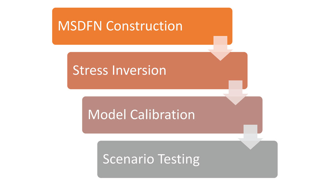
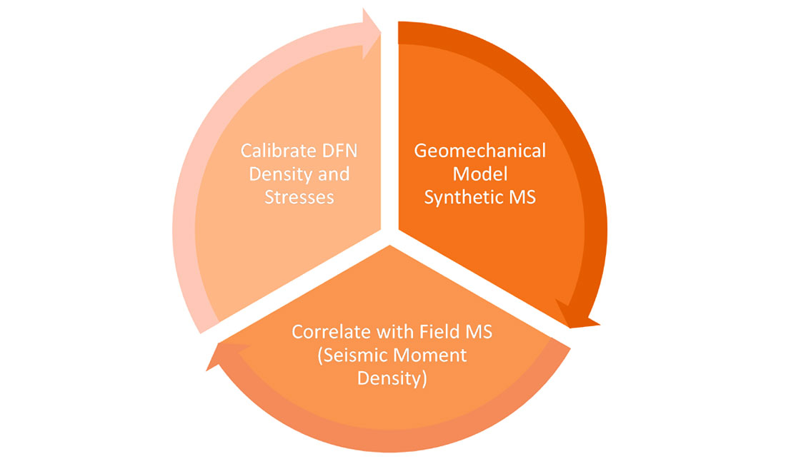
Microseismic geomechanics involves constructing a geomechanical model to predict synthetic microseismicity, for calibration to the field observations. Synthetic microseismic events, including timing, location, source attributes such as magnitude and mechanisms can be estimated from modeled slip or failure resulting from stress and pressure changes associated with the hydraulic fracture growth. Modeled microseismicity then enables a geomechanical interpretation of field data. Figure 1 shows a workflow for a microseismic geomechanics interpretation: including defining a discrete fracture network (DFN) and stress field, calibrating to the microseismic field data, and finally testing alternate designs. The microseismic source mechanisms can be used to help guide the DFN construction and provide details of the stress regime. However, the most important step is the microseismic calibration, as illustrated in Figure 2, which typically involves adjusting the model details (e.g. DFN) to provide a quantitative match between the predicted and observed microseismic using the seismic moment density. Predicted microseismicity is first filtered to the same magnitude sensitivity as the field, and the locations are statistically perturbed based on estimated uncertainty. Another aspect of the calibration is the net pressure, resulting from matching the ‘as pumped’ injection rate and volume. Further details are described below in the context of a Montney case study.

The resulting calibrated model provides a more thorough understanding of the hydraulic fracture network and its representation through the recorded microseismicity. The model is able to distinguish between wet and dry events, as well as reconcile the aseismic and microseismic deformation. The calibrated model provides the reservoir contact (surface area of the fracture network, for example), and models the proppant transport during the injection to provide an estimate of the proppant distribution and hence effective propped portion of the hydraulic fracture. Once calibrated, the model can be used to investigate how the fracture network and associated propped reservoir contact changes with different fracturing or completion scenarios. Virtually testing alternative designs is particularly relevant in the current economic conditions, where statistically testing a sampling of wells with different designs becomes cost prohibitive. Therefore, the microseismic geomechanics interpretation and history match of existing projects is a route to optimize and improve design, thereby extending the microseismic VOI.

Case Study

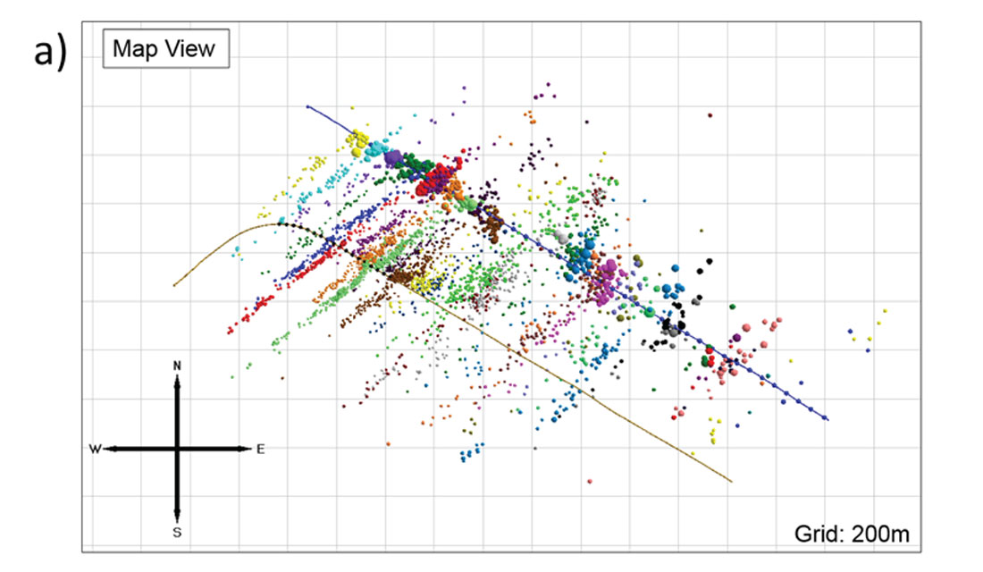
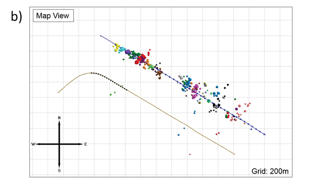
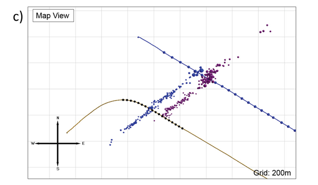
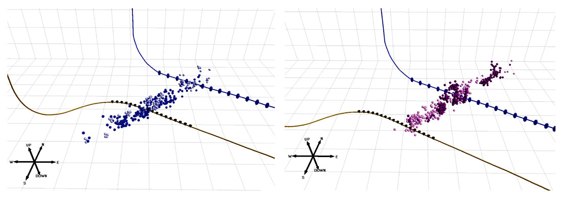
The study examines a Montney open-hole, sliding-sleeve hydraulic stimulation, where microseismicity was recorded from the heel section of a parallel, horizontal well. The spatial distribution of the microseismicity indicates strong planar fractures with asymmetry towards the SW (see Figure 3). The data shows relatively large magnitude events along the treatment well and varying amounts of asymmetric microseismicity for each stage (Figure 3). Stimulations of unconventional reservoirs in the Montney have previously been shown to exhibit asymmetric distribution of the microseismic cloud about the wellbore (Maxwell et al., 2011), potentially impacting reservoir contact. Asymmetric propagation of the hydraulic fracture may be a result of geological structural setting, tectonic stress, pore pressure heterogeneity, or potentially stress shadow from adjacent stages. Detection bias as a result of the monitoring acquisition geometry may introduce apparent asymmetry which can be tested by examining the entire fracture geometry resulting from the total injected volume using a microseismic geomechanical simulation. In this case study, the stage-by-stage variations suggest some stress shadowing component.

Microseismic Geomechanical Model Details

The 3D geomechanical model described here is a fracture-based modeling scheme that is able to quantitatively interpret the hydro-mechanical aspects of fracture propagation and its associated microseismicity. The modeling software package 3DEC has the unique capability of modeling the propagation of the tensile hydraulic fractures along with its interaction with a pre-existing DFN, fully simulating the coupled hydraulic and geomechanical aspects of fracturing (Damjanac and Cundall, 2014). The formulation is a hybrid-continuum, discrete-element based code, coupled with fluid flow within the DFN. An explicit, time-marching, finite-difference scheme is applied to compute the stress and strain of the discrete elements. A discrete element contact law describes the forces and stability of the fractures. Fluid flow within the fracture network is driven by pressure gradients assuming Darcy’s Law laminar flow.

DFN and Initial Stresses

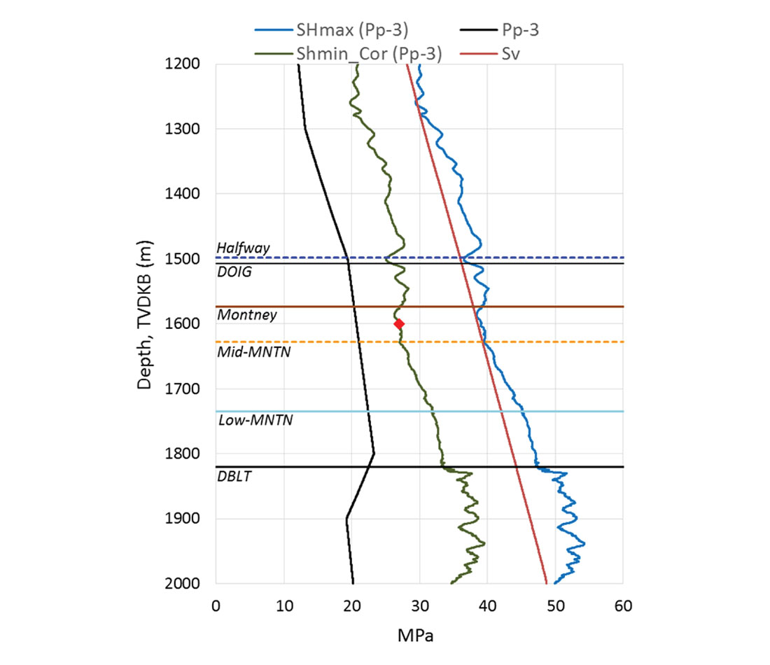
A well constrained geomechanical model requires geologic inputs including elasticity parameters, the stress field, density and fracture characteristics of the DFN. Stress, pore pressure, and mechanical properties are estimated from logging suites and drilling observations. The minimum principal stress is calculated from the Poisson Ratio including corrections due to pore pressure, tectonic stress and closure pressures from DFIT analysis (Figure 4). Flow and build-up tests indicate an over-pressurization in the Montney. The vertical stress is estimated from the density logs and the maximum horizontal stress is estimated by shifting slighting above the vertical stress to maintain a strike-slip (consistent with the microseismic based stress regime defined below).

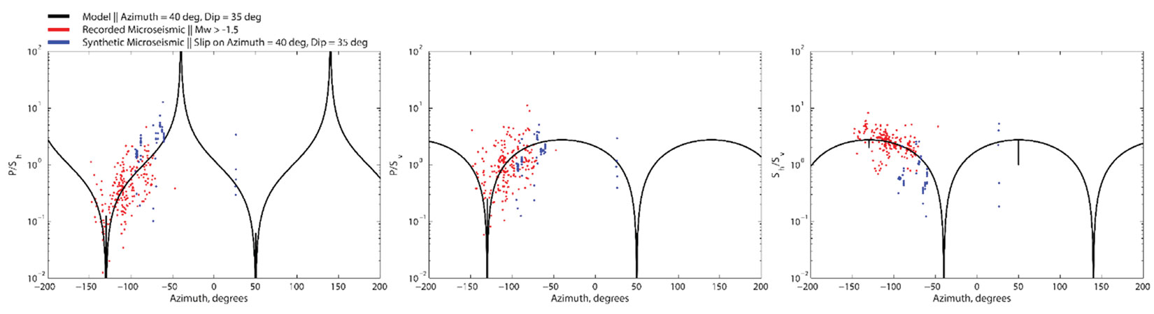
Following QC of the microseismic data, including examination of the magnitude sensitivity and detection biases, it was concluded that the microseismic data shows asymmetric fracture propagation for a number of stages. In addition to the spatial distribution of the microseismicity, amplitude ratios (Sv/Sh, P/Sv, and P/Sh) from double-couple source mechanisms can be used to infer orientations of the DFN (Figure 5). The microseismic data indicates a primary and secondary fracture set associated with the relatively large magnitude, near-well events and the smaller offset events. The fractures are oriented with an azimuth 40 degrees E of N, dip 35 degrees and 87 degrees E of N, dip 35 degrees, respectively. Following Kohli and Zoback (2013), the TOC and clay content is used to estimate joints strength of the DFN.

Hydraulic Fracture Simulation and Microseismic Calibration

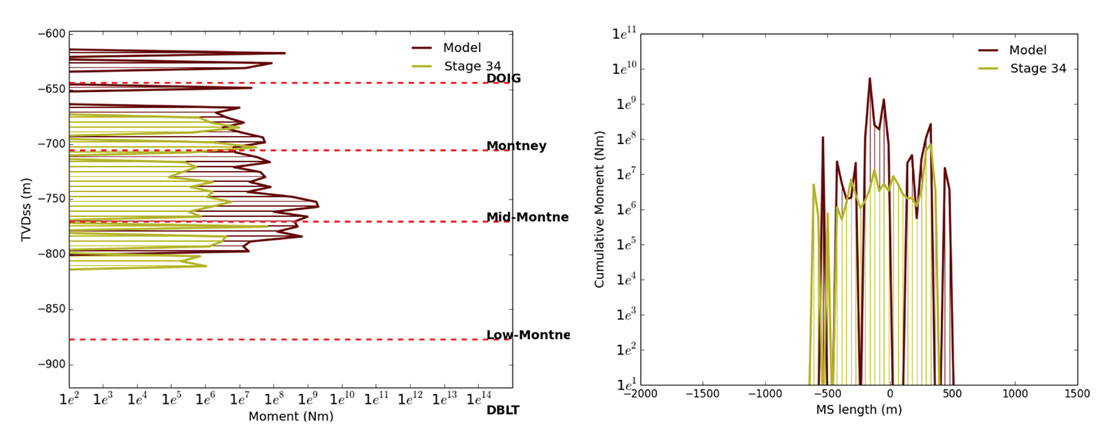
A geomechanical model is populated using the geologic data, DFN orientations, and stress inputs described previously. For each stage, slick water was injected for 33 minutes at a rate of 11m³/min including a 30/50 proppant ramp. Figure 6 shows a comparison of the depth and lateral distribution of seismic moment showing a good match with the field data. The initial model shows a good match to the character of the microseismicity for stage 32 (Figure 7). Applying a horizontal stress gradient results in a close match to the asymmetric stage 34. The simulations show a strong temporal and spatial match in terms of length, width, and height to the field microseismic data suggesting the correct mass balance of fluid and proppant distribution for a single planar hydraulic fracture for each case. In both cases, the fracture lengths and heights are on the order of 1km and 120m respectively. Since the same model can match the fracture geometry of both stages, we conclude that the asymmetry is real and likely a result of a stress shadow interaction between stages.

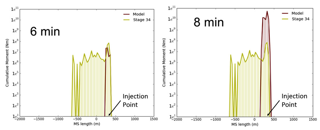
In order to match the relatively large magnitude, near-well events the modeling was also run by initially injecting into a DFN segment. A common assumption with sliding-sleeve completion is that the hydraulic fracture grows from pre-existing fractures intersecting the well. A model was run by injecting into a fracture near the injection point that is oriented at an obtuse angle from the maximum principal stress direction. In this case, shear stress along the joint is most efficiently released and results in a larger seismic moment. Figure 8 illustrates the distribution of seismic moment relative to the injection point, indicating an increase in seismic moment associated with slip along the fracture early in the injection. Therefore, initial injection into a DFN segment is a likely cause of these relatively large magnitude events.

Scenario Testing

The calibrated model can then be used to examine alternate injection and completion scenarios in order to optimize the engineering design. For example, changes to the fracturing fluid system could be examined by changing the fluid viscosity, rate or volume, or a different proppant schedule could be modeled. On the completion side, a plug-and-perf configuration could be tested and the perforation spacing examined, or spacing between fracturing stages adjusted. Well interference can also be examined for various offset well spacings. In each case, the reservoir contact can be assessed by computing the stimulated surface area within the reservoir, potentially limited to some proppant concentration for a measure of the effective propped fracture area. The reservoir contact can then be compared between designs, or alternatively the fracture network can be input into a reservoir simulation to rank potential designs.

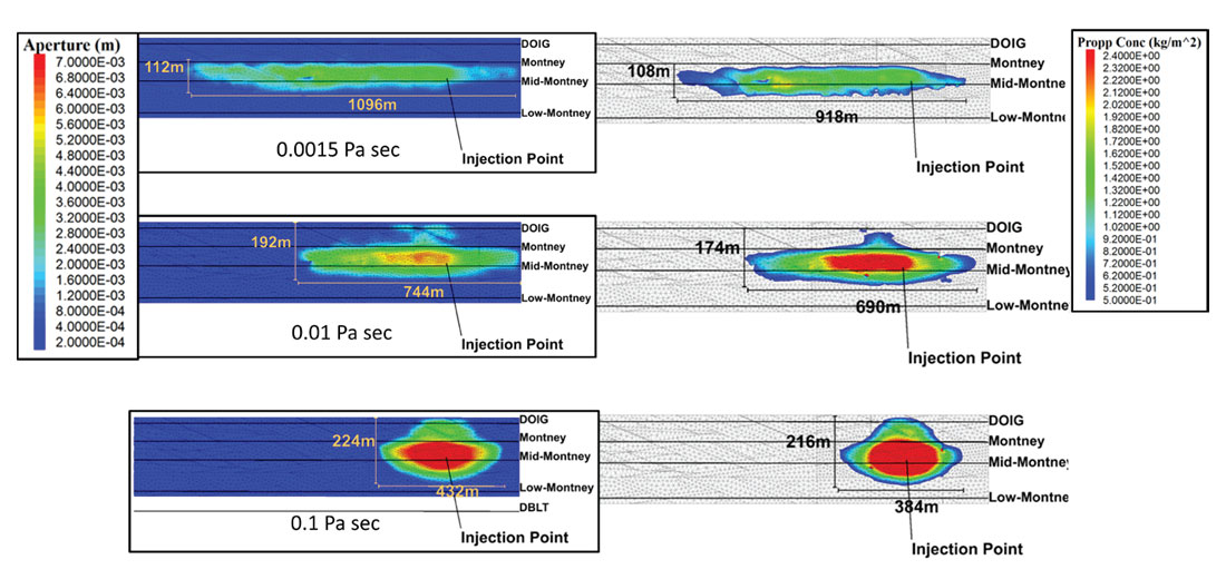
As an example, the calibrated model from this project was simulated using different fluid viscosities (Figure 9). Increasing the viscosity is found to reduce the length growth but causes more height growth. The fracture apeture also increases with viscosity. However, the higher viscosity fluid is also more effective at transporting proppant, resulting in more uniform and increased proppant concentration in the shorter, wider fractures.

Conclusions

In conclusion, the microseismic geomechanical interpretation was used to investigate the complete fracture network. An upper Montney case study was modeled matching the microseismic moment distribution and the overall character of the microseismic images. The model was also used to investigate assymetry in the microseismic images, which found that the injection volume constrained model could replicate fracture geometries of both asymmetric and symmetric stages. The calibrated model was also examined for different engineering designs, specifically increasing the fluid viscosity.

Microseismic geomechanics can therefore provide additional insights from microseismic data. The calibrated model provides additional understanding of the fracture system, including the proppant distribution. The validated model can also be used to examine alternative injection and completion scenarios, thus optimizing the engineering design. The workflow therefore extends the value proposition of existing microseismic data to potentially improve future hydraulic fracturing.