Magnitude Determination, Event Detectability, and Assessing the Effectiveness of Microseismic Monitoring Programs in Petroleum Applications

Introduction

Magnitudes and locations are the first-order output for microseismic events recorded during hydraulic fracture stimulations and longer term reservoir based extraction operations (eg., CSS, SAG-D, CO2 sequestration). The magnitude describes the strength of an event and tells us about the dynamics of the fracturing processes and the distribution of magnitudes outlines the effectiveness of the data acquisition configuration. Although magnitude may seem straight forward to calculate, a number of different magnitude scales have been proposed over the years. Most of these scales are lacking in that they do not relate magnitude to a physical model. The exception is moment magnitude, introduced by Hanks and Kanamori (1979), which can be used to bridge waveform amplitudes to the seismic moment, involving fault area and slip, assuming the recording system is tuned to the appropriate signal bandwidth.

In this paper, we provide a historical perspective on calculating magnitudes, and how from the various magnitude scales the moment magnitude scale was developed. We then discuss the conditions which control the values obtained and the role of instrumentation and bandwidth on the magnitude estimates. We return to moment magnitude and detail what is involved in calculating this quantity. Finally, we touch on the issue of detectability as related to monitoring in the petroleum industry.

A Brief History of Magnitude

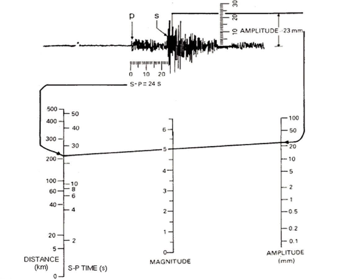
The “Richter Scale” has become a ubiquitous parameter in the public consciousness. Richter (1935) developed the scale for describing the relative strengths of earthquakes in California, and related the amplitude of a waveform recorded with a particular instrument (a Wood-Anderson seismograph) at a given distance from an event to the strength of the event. Figure 1 shows diagrammatically how Richter magnitude is calculated: an amplitude is read from the S-wave and related to a distance, through the temporal separation of the P and S wave, to obtain a magnitude. An increase in 1 of the Richter magnitude corresponds to a factor of 10 increase in the amplitude of the waveforms, and therefore a factor of 30 increase in energy. The logarithmic nature of this scale made the large range of observed magnitudes more palatable for the public audience.

Since then, there have been a number of similar magnitude scales in the literature. Some are tailored to a particular region with slightly different calibration curves (to account for differences in seismic attenuation, geological province, etc.), which are referred to as local magnitudes. Further complicating matters was that depending on the exact waveform used to determine amplitude, different calibrations need to be employed to arrive at a relatively standardized magnitude measurement. Gutenburg and Richter (1936), for example, used the amplitude of teleseismic 20s surface waves to derive a magnitude scale for crustal earthquakes. These relationships, for local magnitude determination, can be summarized as:

Magnitude = log10 (Amplitude) + CorrectionFactor

where the correction factor depends on distance and sometimes the period of the waveform. This balkanization of magnitude scales is still reflected in global earthquake catalogues, although in their discussion of these matters Aki and Richards (2002) note optimistically:

“The fact that a seismic event may have different magnitudes on different scales ... is in practice the basis for methods of identifying the event (perhaps as an earthquake or an explosion). Thus, rather than seeing different magnitude scales as an inconvenience, they can be viewed as a useful means for characterizing the great variety of seismic signals.”

Such a study was conducted recently by Bormann et al. (2009) discussing the interrelations between different magnitude scales to earthquake data recorded in China.

However, there are a couple problems with such magnitude scales: one is that they are unabashedly empirical, there is no tie to a physical model so a given magnitude cannot be explicitly related to any parameters of the fault; the other problem is more practical, that these magnitude scales are saturated for the largest earthquakes. Kanamori (1977) and Hanks and Kanamori (1979) developed the moment magnitude scale to address these shortcomings. The seismic moment M₀, is based on a model assuming shear displacement of a planar fault, and is the product of the shear modulus, μ, the average slip on the fault, d, and the area of the fault, A. By measuring the energy, E, in the waveforms, they related this quantity to the seismic moment through the approximate relation:

and then developed a scale from this measurement that roughly matched the unsaturated part of the magnitude scale. Although this scale was developed specifically for the largest of earthquakes, its range of applicability extends all the way down into the microseismic realm.

Magnitudes and Instrumentation

Because of the band-limited nature of seismic signals, the design of the recording system is an important consideration in any discussion of magnitude. The corner frequency of an event is empirically related to the magnitude of the event. The relationship arises from the relationship of seismic moment to the area of a fault surface: a larger area fault surface gives rise to a larger wavelength and therefore lower frequency signals whereas small area faults give rise to higher frequencies. The corner frequency can thus be viewed as the characteristic or natural frequency of the event. Microseisms, in the magnitude range of -3 to 0, give rise to corner frequencies in the range of approximately 50 to 500 Hz as they occur on fractures with dimensions of 10s of cm to a few metres. Macroseisms, with magnitudes of 0 to 5, occur on larger faults (10s to 100s of metres) leading to low corner frequencies in the range of 1 to 50 Hz. The largest earthquakes, for example the 2004 Great Sumatran Earthquake, cause slips on fault planes on the order of 1000 km, resulting in very low frequency corner frequencies (in this case, as summarized by Menke et al., 2006, 2 mHz or about an 8 minute period).

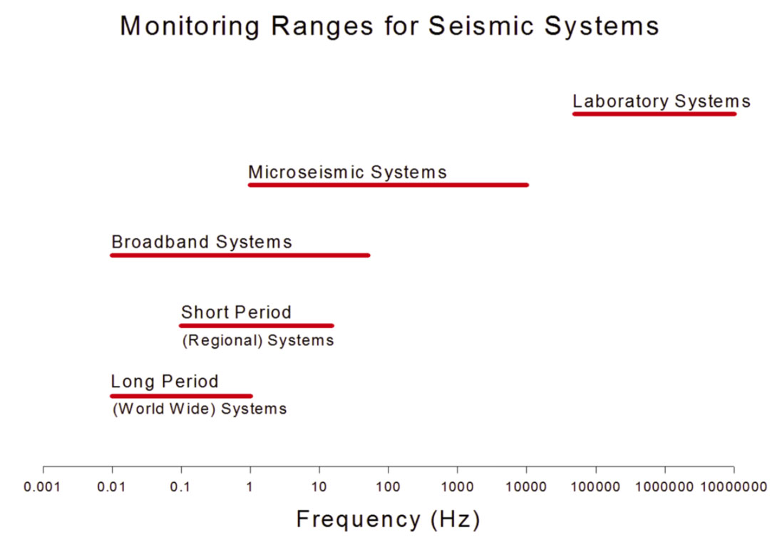
As seismicity occurs over a broad range of magnitudes, sensing earthquake in the corresponding bandwidths requires different instrumentation. Figure 2 summarizes the ranges of application for various seismic instruments. From the smallest transducers to the measure the MHz signals in ultrasonic experiments to the broadband seismometers that measure signals with periods of minutes, there is a corresponding span in magnitudes from -4 to 9. Each of the sensors described in Figure 2 are designed to have a flat frequency response over a given bandwidth, which can be read as a prescribed frequency range. Events with bandwidths outside of the flat frequency reponse will be distorted by the instrumental response and yield unreliable magnitude estimates if they are detected at all.

The bandwidth of the instrument needs to capture not just the corner frequency, but a robust estimate of the spectral plateau, and the high-frequency decay. This last requirement practically means being able to sample at a rate that is about a factor of 8 greater than the corner frequency. For microseismic events, with magnitudes down to -2, corner frequencies can be 500 Hz and therefore sample rates of 4000 Hz.

Moment Magnitude

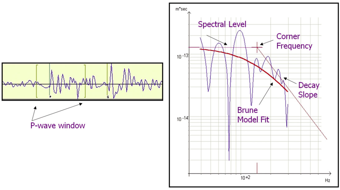
The signal from three component sensors can be inverted for seismic moment by assuming a model for the source and relating that to a rupture area and an amount of slip. The Brune model for the displacement (Brune, 1970) stipulates that frequency response of the signal is flat until the corner frequency is reached, at which point, the amplitude falls off as f ⁻², although other models yield high-frequency asymptotes of f ^−2.5 or f ⁻³. By fitting such a model to the displacement spectrum, as in Figure 3, the low-frequency plateau | W_c | can be estimated and used directly in the calculation of seismic moment as this relates to the area of slip on the fracture plane. Also entering the equation are geometrical spreading, R, wave-speed c, the density of the rock p, and a factor for the radiation pattern imposed by the moment tensor, F_c :

This equation has been generalized to measurements of either the P, or S wavefield; for P waves | W_c | = | W_p | and for S waves

Boore and Boatwright (1984) developed a rough estimate for F_c if one cannot adequately determine the radiation pattern of the moment tensor, F_p=0.52 for P waves and F_s=0.63 for S waves. The right side of the equation relates to parameters of the faulting process: μ is the shear modulus of the rock, d̄ is the average displacement of the fault, and A is the area of the fault. With seismic moment, measured in Nm, we can then determine moment magnitude from the following formula:

In contrast to the empirical relations discussed earlier, this definition links magnitude to the properties of the fault. The constants in the above relation ensure that moment magnitude falls in a range that is comparable to other magnitude scales and makes it a logical choice for use with microseisms.

Event Detectability

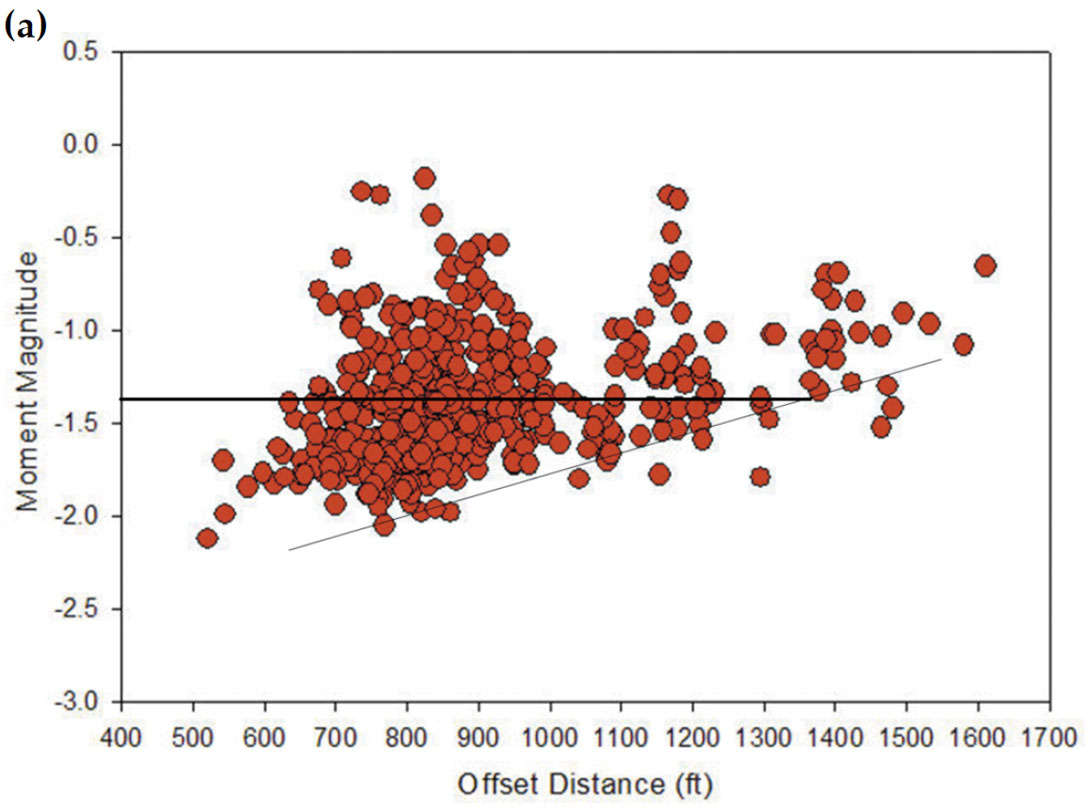
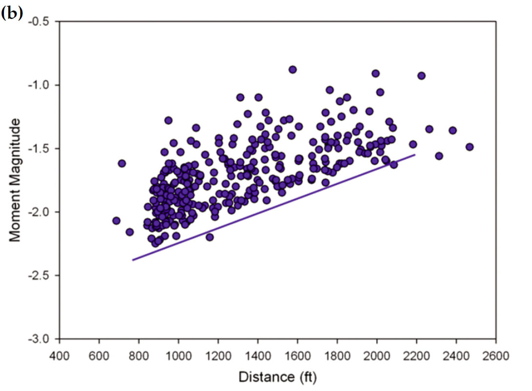
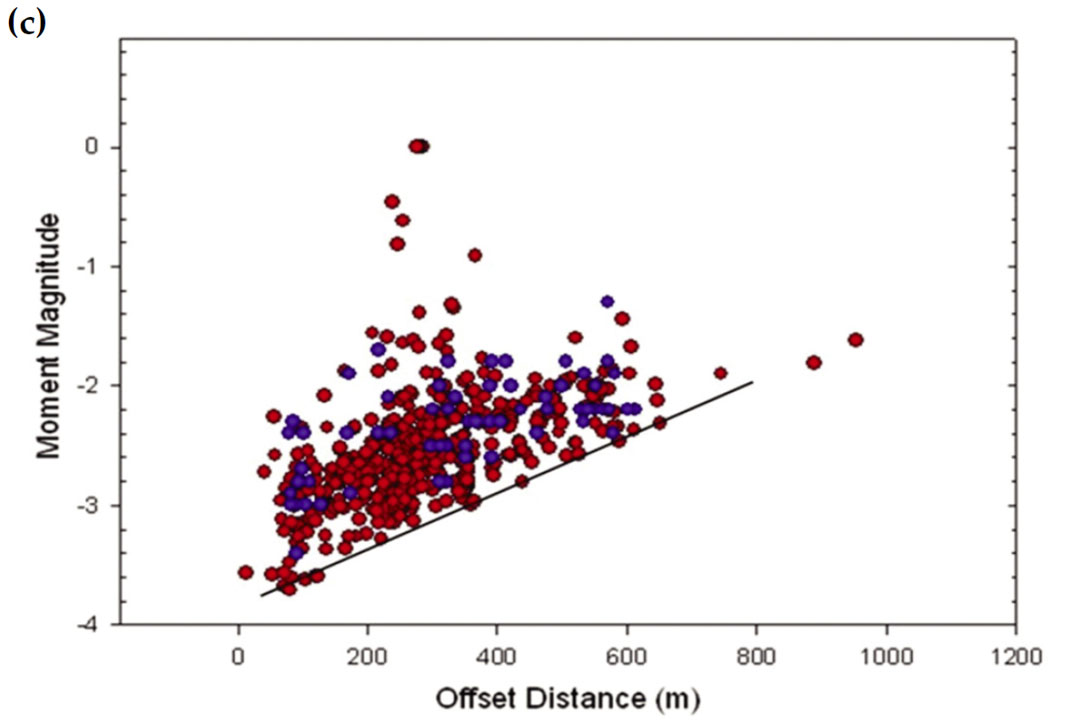
The moment magnitude controls the range of detectability of microseismic events and is, therefore, a very important consideration in determining how a treatment should be monitored. In Figure 4, we plot a number of scatterplots of magnitude versus distance (from the centre position of the downhole observation array) for different environments. Figure 4a shows the magnitude versus distance plot for a hydraulic fracture in a shale formation. The minimum detectable magnitude (black line) appears to generally increase monotonically with distance. For data completeness, as represented by the horizontal line, there is an equal probability of detecting an event of M_W > -1.4 over the entire volume of interest. The distribution also suggests events were only detectable to a distance of approximately 1600 ft from the observation array. In this case, unbiased interpretation can only be provided by considering the complete data set. In Figure 4b we show the magnitude-distance distribution for events from a hydraulic fracture in a tight gas sand formation. Outside of hydraulic fractures, Figure 4c shows the results of two stages of a multiple-year cyclic steam injection program. Again, it is clear the minimum detectable magnitude increases with distance and similar to the shale example, appropriate data completeness can be assigned. In the CS example, bias is observed throughout the volume of interest, suggesting caution be used in any interpretation of the data.

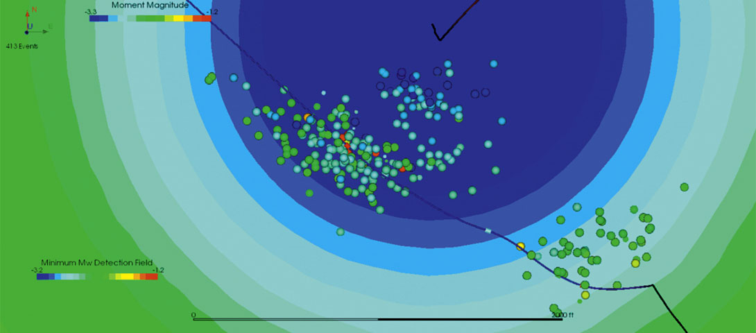
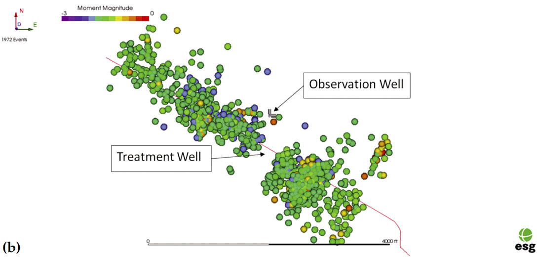
The magnitude distance relationship dictates the optimal placement of the sensor arrays. In order to ensure detection of events of a certain size, an a priori estimate of the minimum detectable magnitude curve is necessary to verify the sensor geometry. Figure 5 shows such a figure, for a hydraulic fracture in chalk. The colour scale of the contours is the minimum detectable magnitude, starting at blue for smaller magnitudes near the observation well, going to hotter colors for larger magnitudes further out. Also on this image are the events recorded from the treatment, with the same moment magnitude colour scale for the events. Nowhere in this example are the event colors cooler than the underlying contours, indicating that although lower magnitude events are certainly present far from the well, they are undetectable to the weaker signal to noise ratios they yield.

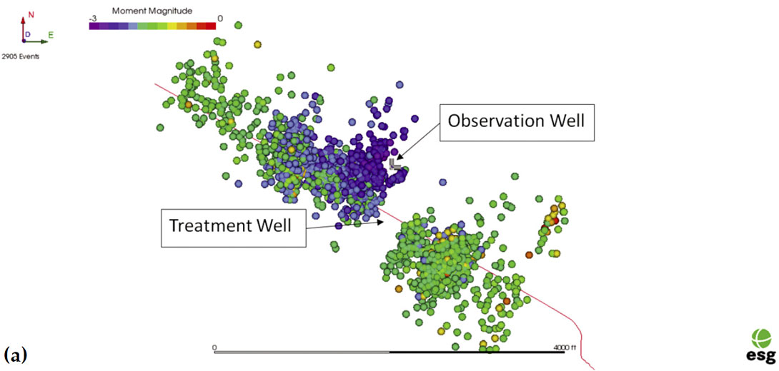
As discussed in Figure 4, one implication of the slope of the minimum detectable magnitudes is that without considering the magnitudes of the observed events, one might get a biased estimate of the fracture geometry. In Figure 6a, we show the distribution of all events recorded from a hydraulic fracture in shales. There is apparently growth out from the horizontal treatment well beyond the observation well. However, by examining the moment magnitudes of the events comprising this apparent growth, we observe they are of a very low magnitude. By considering only those events representing the minimum magnitude that can be observed across the entire dataset, in this case at M_W =−1.8, we can define a complete data set for the volume. By excluding events below this threshold, we homogenize the data and we see that, in Figure 6b, the low-magnitude tongue of events beyond the observation well has disappeared. So we can conclude the stages comprising these low-magnitude events are not exceptional compared to the further stages which were too far out for similar low-magnitude events to be registered.

Discussion

Magnitude is a quantity which is intuitively obvious at first glance, but nuanced and complex upon further inspection. With the panoply of arbitrary magnitude scales, only relative magnitudes within the same scale will be truly meaningful in most cases. Moment magnitude uniquely speaks to the physics of the fracture though the seismic moment, and for this reason, should be considered above all the other magnitude scales in the microseismic regime. The instrumental dependence of the magnitude calculation needs to be considered as well: although it is one number, accurate determination of the magnitude is only possible with a full sampling of the low- and high-frequency asypmtotes of the spectrum and therefore we need to measure the seismicity with instruments tuned to the expected magnitude range. For microseismic events, the bandwidth of the instruments needs to capture corner frequencies in the range of 100 to 500 Hz, consequently sampling rates need to be at least 4000 Hz to accurately calculate the moment magnitude. The moment magnitude is very relevant in monitoring in the petroleum industry in determining the optimal placement of observation arrays. As the minimum detectable magnitude increases with observation distance, there are frequently many more low-magnitude events near the sensors, which could lead to a biased estimate of the effectiveness of the treatment in this zone. Homogenizing the data by removing events below a threshold moment magnitude can remedy this problem and give a consistent image of the microseismicity for interpretation.