It’s the Fluids that Count

Fluid Properties and Their Geophysical Signature

Locating and identifying pore fluids is usually the ultimate goal of any geophysical activity. This not only involves oil and gas recovery, but also assessing ground water resources and tracking pollution plumes. As we strive to make geophysical methods, particularly seismic results, more quantitative, we must have a thorough understanding of the pore fluids and how they interact with the rock. Otherwise, seismic images remain just seismic images and are of limited use to engineers in ascertaining reservoir conditions. Here we will focus on the various pore fluid types and their important geophysical properties.

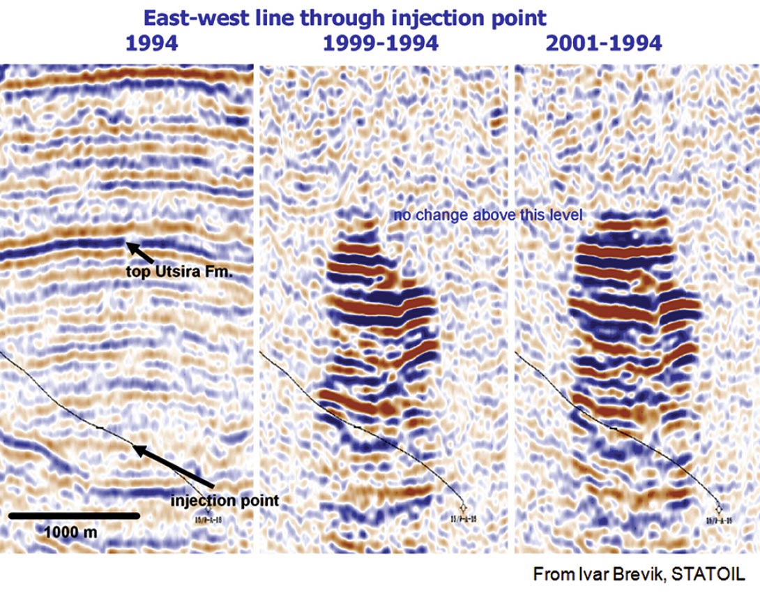
Time-lapse seismic monitoring of reservoir processes is one obvious way to track fluids. In some cases, this fluid response is not subtle. Figure 1 shows the time-lapse response of CO₂ injection in the North Sea. Under the proper conditions, and for the appropriate fluids, changes are easy to detect. The next step is to extract actual fluid properties, identify the fluids, and estimate saturations.

Pore fluids vary widely in composition and properties. At one extreme are light gases with very low densities, modulus and velocity. Heavy oils, on the other hand, can effectively be solids, capable of transmitting shear waves or even supporting the “rock” as the bulk matrix. Brines are the most common pore fluid, and they vary greatly, primarily depending on the salt content. Assuming simple, constant properties is a mistake. Fortunately, most of the important properties vary in simple systematic ways. Realistic properties can be derived with a good estimate of local pressure and temperature conditions and an estimate of composition.

The effect of pore fluid on rock velocity has been documented for many years. The shear velocity changes little, or even decreases slightly with brine saturation. In contrast, the Vp increases significantly after brine saturation. This increase in Vp will be a function of the rock coupled with the fluid properties. The influence of pore fluids is often modeled using Gassmann’s (1951) equations. The fluid changes the saturated bulk modulus of the rock and is related to the difference between the fluid and the mineral bulk moduli coupled through the porosity. These parameters are not all independent, and these terms interact and simplifications and generalizations can be made.

Brines

The great bulk of the pore fluids consists of brines. Their composition can range from almost pure water to saturated saline solutions. Regions with extensive salt in the stratigraphic column often have rapid increases in salinity in the brines with increasing depth. In other areas, the concentrations are often lower but can vary drastically between adjacent fields.

The thermodynamic properties of aqueous solutions have been studied in detail. Utilizing all these data, simple polynomials can be constructed that will adequately calculate the density and bulk modulus of sodium chloride solutions and details were presented in Batzle and Wang (1992).

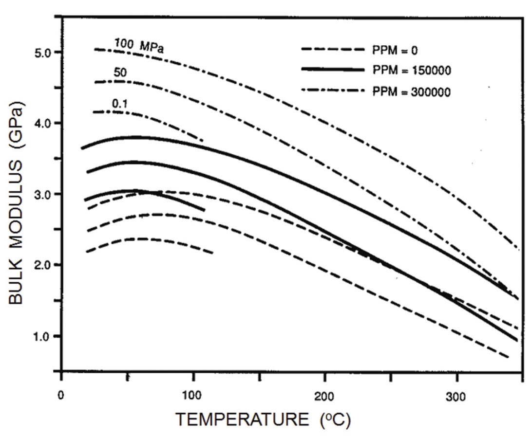
A vast amount of acoustic data is available for brines, but generally for pressure, temperature, and salinity expected under oceanic conditions under which the primary exploration targets were Russian submarines. As might be expected, the bulk modulus increases with increasing pressure and salinity (Figure 2). At high temperatures, water acts as a “normal” liquid, with the modulus (and velocity) decreasing with increasing temperature. Water is unusual in that the bulk modulus reaches a maximum around 60 degrees C and then decreases with decreasing temperature.

Hydrocarbons

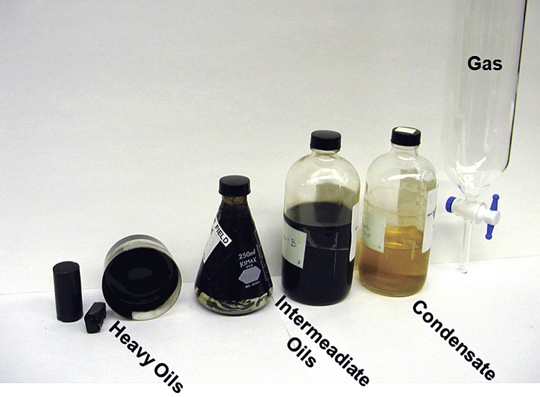
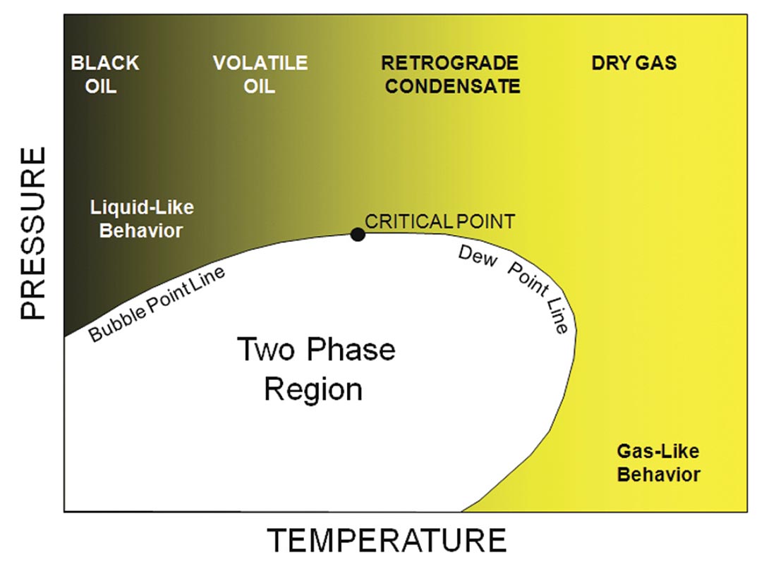
Properties can change substantially for different hydrocarbons and hydrocarbon mixtures. Figure 3 shows some examples of the hydrocarbon family. Figure 4 shows a generalized phase diagram for hydrocarbon mixtures. Velocities and densities will be high (close to water) for heavy ‘black’ oils and decrease dramatically as we move right toward lighter compounds. High pressures and low temperatures result in a glassy or quazi-solid phase. Mixtures, such as oils, have a complex behavior. In many cases, the hydrocarbons are above critical pressure and temperature conditions (above critical point). Properties then can vary continuously from liquid-like for oils with gas in solution to gaslike for mixtures of light molecular weight. As an example, if we start in the single phase, low temperature region, as temperature drops we encounter the bubble point line and gas comes out of solution. At higher temperatures, the dew point line would be crossed, and gas will drop out of solution. Encountering phase boundaries can result in abrupt changes in fluid mixture properties and often are the strongest geophysical signature.

Crude oils can be mixtures of extremely complex organic compounds. Under room conditions, the densities can vary from 0.5 gm/cc to greater than 1 gm/cc with most produced oils in the 0.7 to 0.8 gm/cc range. The American Petroleum Institute (API) number is defined as

API = 141.4/ - 131.5.

This results in API numbers of about 5 for very heavy oils to near 100 for light condensates. The extreme variations in composition and ability to absorb gases produce greater variations in the seismic properties of oils.

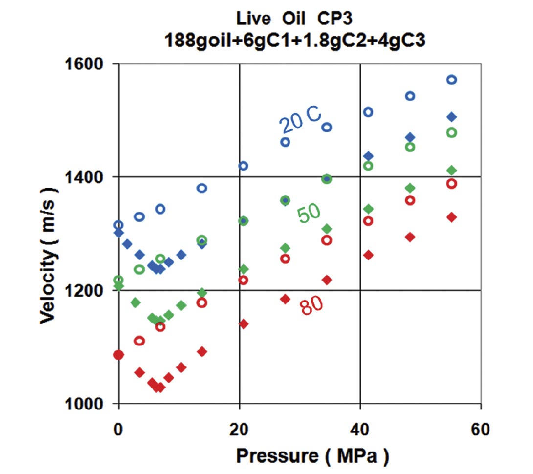
The typical behavior for a light oil with pressure and temperature can be seen in Figure 5. As presure increases, the compressional velocity also increases. However, increasing temperature decreases the velocity. Another important feature is that gas can go into solution in large quanities. Oils without solution gas are termed “dead” oils (open symbols in Figure 5), those with gas in solution are called “live” oils (solid symbols). Putting gas in solution effectively lightens the oil and lowers the velocity. Note that as the pressure is dropped for the live oil, the bubble point is reached at about 7 MPa. Gas starts coming out of solution and the liquid velocity increases (only the liquid phase is being measured in this experiment).

Heavy Oils

Heavy oils are defined as having high densities and extremely high viscosities. Our definition here is for oils with an API less than 10 (density greater than 1 g/cc). These are an abundant resource, particularly here in Canada.

Heavy oils themselves are often fundamentally different chemical mixtures from more typical crude oils due to biodegradation. Straight alkane chains tend to be consumed by bacteria, leaving a mixture of complex organic compounds. This process requires both relatively low temperatures and contact with circulating fresh water. Heavier compounds include asphaltines, bitumens, pyrobitumens, resins, etc. These complex compounds are often rather operationally defined. For example, asphaltines are usually defined as the component of crude oils not soluble in heated heptane. Although this is useful in assessing if solids will form in production pipes, it gives little insight into their physical properties.

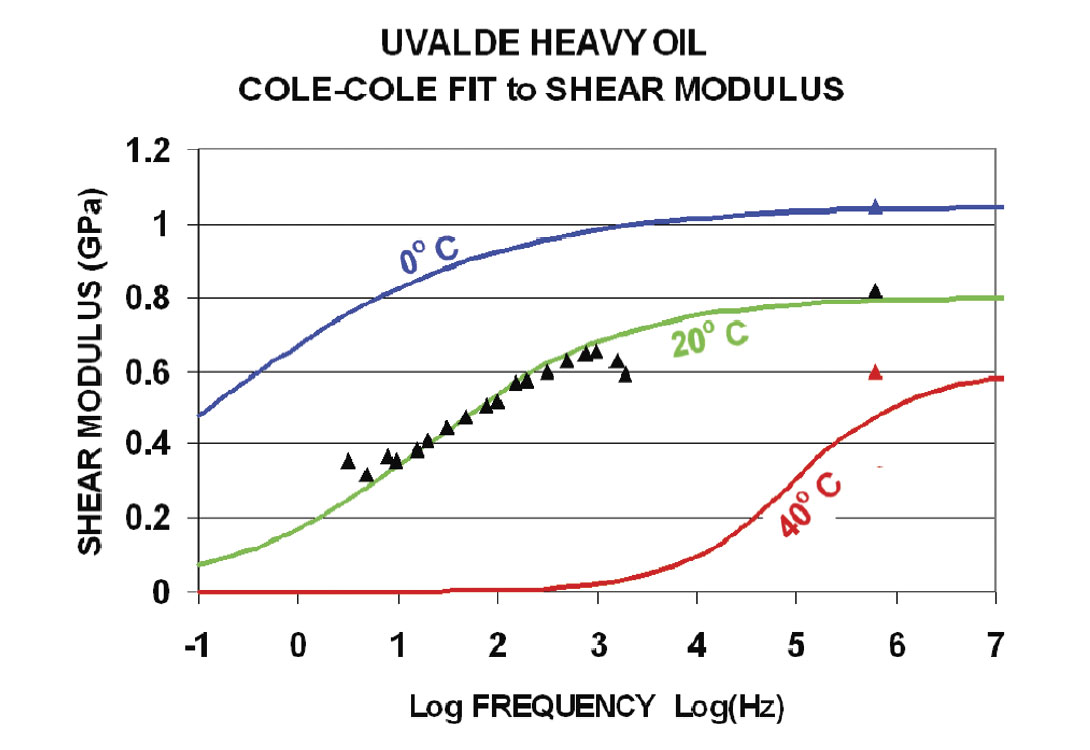
One of the primary features of very heavy oils is that they have extremely high viscosity and begin to act like a solid. This means that these quazi-solids will have a shear modulus and behave viscoelastically. However, one of the features of this viscoelasticity is both a strong frequency dependence as well as a temperature dependence. An example of measured shear modulus versus frequency for a very heavy oil (API = -5) is seen in Figure 6. Note that the frequency is on a logarithmic scale. Here it is obvious that properties measured in the seismic band will not equal those collected with the standard sonic tools nor equal those collected in the laboratory at typical ultrasonic frequencies.

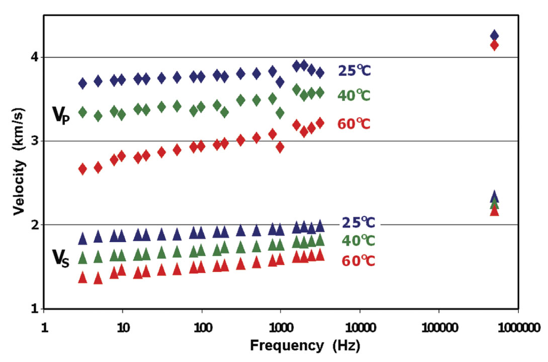
As an example of the influence of heavy oils on the seismic properties of rocks, we can examine the results for a carbonate from south Texas saturated with the very heavy oil seen in Figure 6. As expected the rock velocities are now strongly temperature and frequency dependent. Figure 7 shows that at ultrasonic frequencies, the velocities remain high, even at elevated temperature. However, at low, seismic frequencies, the velocity is much more strongly temperature sensitive. Here, strong velocity dispersion can be seen, even within the seismic band. A similar amount of dispersion was observed by Schmitt (1999) when he compared sonic velocities with those collected by VSP. For these heavy oils, disagreements of more than 20% between seismic and logging frequencies can be expected. Note that in any synthetic modeling of these reservoirs, the reflections of the heavy oil sands based on standard sonic logs would be completely different than the low frequency seismic response.

Conclusions

• Fluids are our primary exploration and monitoring target
• Properties vary dramatically, but systematically with composition, pressure and temperature
• Phase changes can be the most dramatic geophysical signature
• Heavy oils act viscoelastically and velocities measured in the seismic band will not match those measured in well logs or in ultrasonic laboratory tests.