Interpreting fractures through 3D seismic discontinuity attributes and their visualization

Summary

Fractures can enhance permeability in reservoirs and hence impact the productivity and recovery efficiency from them. Fold and fault geometries, stratal architecture and large-scale depositional elements (e.g. channels, incised valley-fill and turbidite fan complexes) are often difficult to see clearly on vertical and horizontal slices through seismic reflection data. Seismic discontinuity attributes help us in characterizing stratigraphic features that may comprise reservoirs and form integral part of most interpretation projects completed today. Coherence and curvature are two important seismic attributes that are used for such analysis. However, for extracting accurate information from seismic attributes, the input seismic data needs to be conditioned optimally. This includes noise removal, using robust dip-steering options and superior algorithms for computation of seismic attributes.

Curvature attributes in particular exhibit detailed patterns for fracture networks that can be correlated with image logs and production data to ascertain their authenticity. One way to do this correlation is to manually pick the lineaments seen on the curvature displays for a localized area around the borehole, and then transform these lineaments into rose diagrams to compare with similar rose diagrams obtained from image logs. Favourable comparison of these rose diagrams lends confidence in the interpretation of fractures. Another way is to generate automated 3D rose diagrams from seismic attributes and correlate them with other lineaments seen on the coherence attribute for example. Finally, volume visualization of stratigraphic features is a great aid in 3D seismic interpretation and can be greatly aided by adopting cross-plotting of seismic discontinuity attributes in the interpretation workflow.

Introduction

Characterization of fractures is essentially the understanding of fracture patterns, so that appropriate ways can be devised for effectively draining out fractured reservoirs. The presence of naturally occurring fracture networks can lead to unpredictable heterogeneity within many reservoirs. Alternatively, fractures provide high permeability pathways that can be exploited to extract reserves stored in otherwise low permeability matrix rock. Consequently, the detection and characterization of fractures is of great interest which is driving significant improvements in azimuthal AVO, image-log breakout interpretation, and seismic attribute analysis. Surface seismic data has long been used for detecting faults and large fractures, but recent developments in seismic attribute analysis have shown promise in identifying groups of closely spaced fractures or interconnected fracture networks.

Coherence and curvature attributes for fracture detection

The coherence attribute has been used for detection of faults and fractures over the last several years. With the evolution of the eigen-decomposition algorithms, coherence is able to further improve the lateral resolution and produce relatively sharp and crisp definition for faults and fractures. However, volume curvature attributes have shown promise in helping us with fracture characterization (Al-Dossary and Marfurt, 2006; Chopra and Marfurt, 2007a and b, 2008). By first estimating the volumetric reflector dip and azimuth that represents the best single dip for each sample in the volume, followed by computation of curvature from adjacent measures of dip and azimuth, a full 3D volume of curvature values is produced. There are many curvature measures that can be computed, but the most-positive and most-negative curvature measures are the most useful in mapping subtle flexures and folds associated with fractures in deformed strata. In addition to faults and fractures, stratigraphic features such as levees and bars and diagenetic features such a karst collapse and hydrothermally-altered dolomites also appear to be well-defined on curvature displays.

Multi-spectral curvature estimates introduced by Bergbauer et al (2003) and extended to volumetric calculations by Al Dossary and Marfurt (2006) can yield both long and short wavelength curvature images, allowing an interpreter to enhance geologic features having different scales. Tight (short-wavelength) curvature often enhances subtle flexures on the scale of 100-200 traces that are difficult to see in conventional seismic, but are often correlated to fracture zones that are below seismic resolution, as well as to collapse features and diagenetic alterations that result in broader bowls.

The quality of these attributes is directly proportional to the quality of the input seismic data. So for extracting more accurate information from seismic attributes, the input seismic data needs to be optimally processed. The term ‘optimally’ essentially means that any or all distortion effects, whether near-surface, or amplitude/phase related, or others are taken care of during processing if not totally eliminated. When such prestack or poststack data are loaded on workstations, they may still show a certain amount of noise level. This noise could be of various sorts – acquisition related, processing artifacts or random. We recommend three important considerations for computation of geometric attributes taking coherence attribute as an example. These three considerations are (a) data conditioning, (b) using dip-steering for data with reflector dips, and (c) the choice of algorithm employed for attribute computation. Application of structure-oriented filtering run on seismic data sharpens the subsurface features of interest and tones down the background noise. Coherence attribute generated on such seismic volumes yields crisper features. Dip-steering option when used in coherence computation results in clearer looking volumes that are devoid of any structural contour patterns and so prevent misleading information. Finally, a coherence algorithm based on the method of eigen-decomposition of covariant matrices called energy-ratio algorithm, demonstrates superior performance than other available algorithms.

Visualizing seismic attributes

Fold and fault geometries, stratal architecture and large-scale depositional elements (e.g. channels, incised valley-fill and turbidite fan complexes) are often difficult to see clearly on vertical and horizontal slices through the seismic reflection data (Kerr, 2003). Consequently, visualization techniques are used for viewing the data, whether it’s the input seismic data or derived data in terms of seismic attributes. It is important because it helps extract meaningful information, allows for greater interpretation accuracy and improves efficiency. Traditional 2D interpretation workflows consisted of picking faults and horizons on dip and strike lines to generate the time and structure maps through gridding and contouring. With the advent of 3D data, this interpretation workflow was morphed into picking, say, every 10th inline and 10th crossline. Later improvements included interpreting on time slices and the use of automatic picking algorithms (e.g. Rijks and Jauffred, 1991). Important drilling decisions are based on these maps that entail huge financial investments.

3D visualization of seismic data is also an efficient way of displaying structural or stratigraphic hydrocarbon traps in their true three-dimensional perspective, allowing interpreters to comprehend the complex geometric inter-relations of horizons with faults and deviated well penetrations. 3D volume rendering is one form of visualization that involves opacity control to view the features of interest ‘inside’ the 3D volume. The interpreter chooses a seismic amplitude or attribute subvolume of interest, interactively adjusts and applies the opacity, thereby delineating geologic features of interest in their true disposition. All this can be done rapidly providing insight about the details on the shapes, and highlighting depositional features such as channels and buildups. Such 3D visualization significantly augments the understanding of features seen on vertical sections and maps.

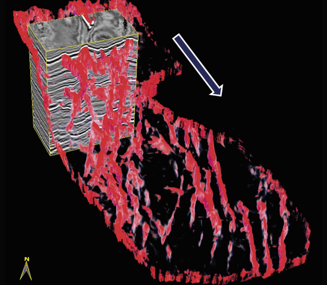
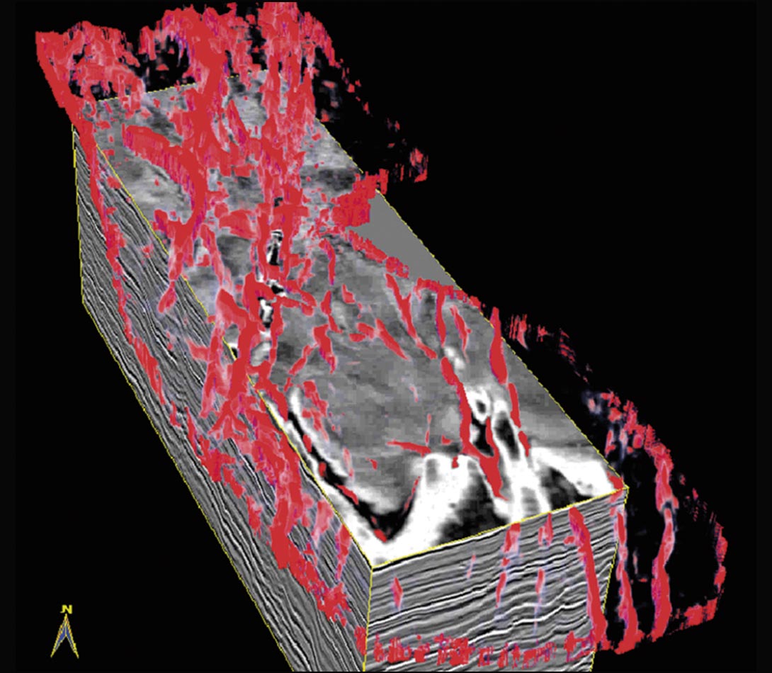
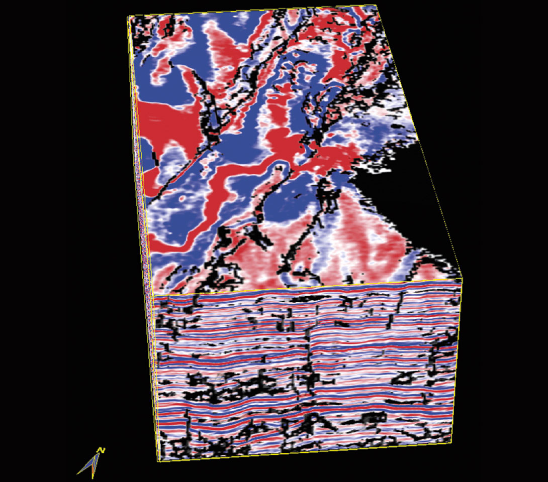
For this reason, a judicious choice of opacity in the attribute subvolume can help in its correlation with the seismic volume. If fault correlation in the zone of interest is the objective, a useful feature that would be utilized is shown in Figure 1. First we generate a strat-cube encompassing the zone of interest from the most-positive curvature attribute volume. Then, using opacity control features, we retain only the high values displayed in red resulting in the fault skeleton which we overlay on the seismic volume for visual correlation. Animation of the seismic inlines in the direction of the white arrow helps the interpreter determine whether the vertical red planes represent faults, axial planes of tight anticlines, or artifacts introduced through acquisition and processing. Once this is checked, similar animation should be carried out in the crossline and time slice direction (Figure 2).

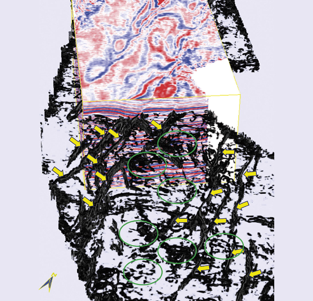
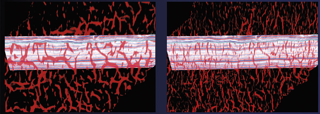
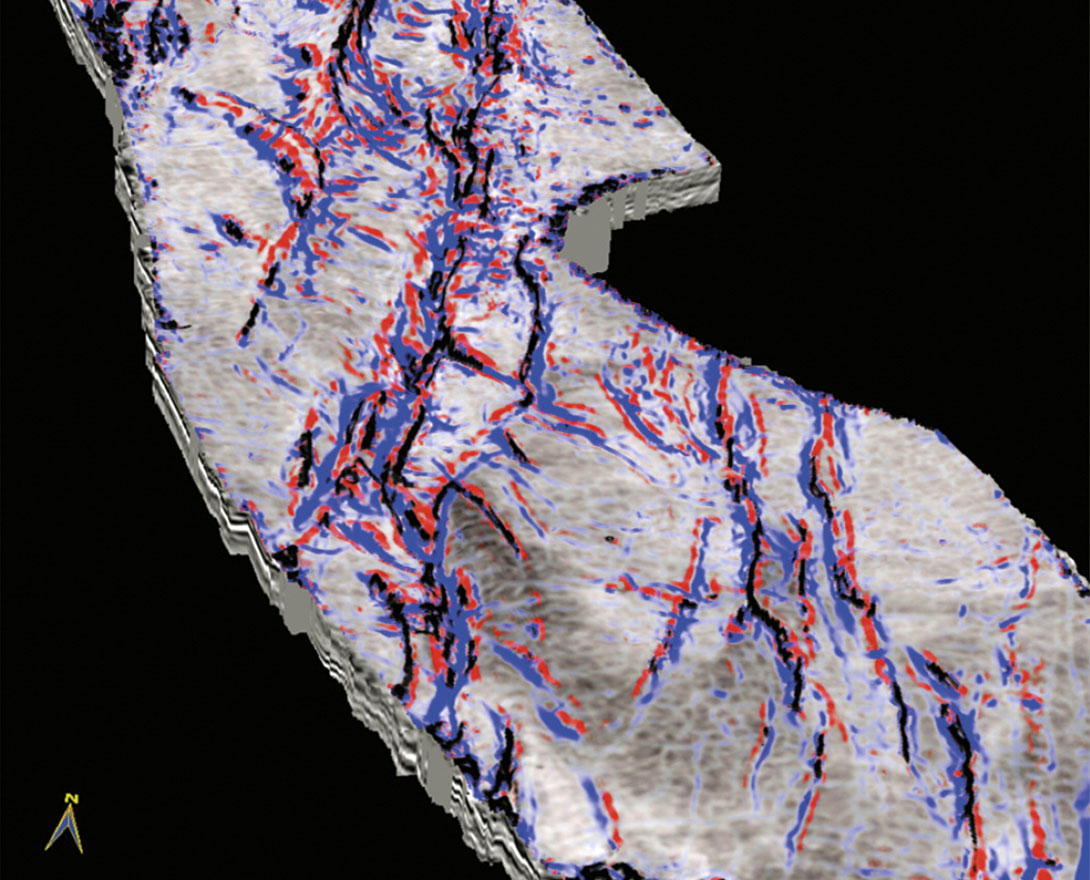
In Figure 3 we show the correlation of the seismic signatures with the faults as seen on the stratal coherence skeleton. Notice that in addition to the main faults (some indicated with yellow arrows) which stand out clearly, there are a number of low coherence features (some shown with green circles) which not only clutter the display but create problems in a straightforward interpretation of these faults. It is possible to get rid of such unwanted features with the help of crossplotting of attributes discussed in the next section. In Figure 4 we show a similar correlation of seismic with both strata long and short wavelength most-positive curvature skeletons. Notice that while the large faults and fractures are seen clearly on the long-wavelength most-positive curvature display, finer/crisper detail can be seen on the shortwavelength most-positive curvature strata display.

Multi-volume rendering

The previous workflow involved displaying an attribute volume with opacity controls and with opaque seismic lines and time slices. We are also able to view multiple 3D volumes within the same congruent 3D space. We find co-rendering coherence or the most-positive (or depending on the geologic features of interest, most-negative) curvature volumes with the seismic amplitude volume as being particularly useful. Figure 5 shows a coherence volume showing on the low coherence features (high coherence values made transparent) co-rendered with the seismic volume. For curvature attributes also the high (for most-positive curvature) or low (for most-negative curvature) curvature values can be set to be opaque and the other values transparent. These attributes would serve as a guide, while interpreting. Figure 6 shows such a visualization, where the coherence (low values in black), mostpositive curvature (high values in red), and most-negative curvature (high negative values in blue) attributes are co-rendered with the seismic volume in a strat-cube. Notice, in one single composite display it is possible to interpret the seismic change in the waveform discontinuities (black), the upthrown edges of the fault blocks (red) and the downthrown sides of the fault blocks (blue).

Cross-plotting for visualizing faults/fractures

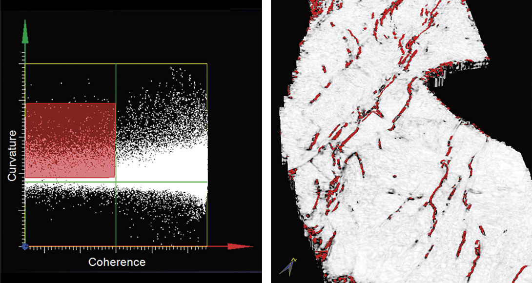
Cross-plotting is routinely used in well-log and AVO analysis, as it provides a visual means for a human interpreter to see trends and correlations between mathematically independent measures that are correlated through the underlying geology. Since coherence (which is a measure of waveform discontinuity) and curvature (which is a measure of structural deformation) are mathematically independent attributes that can be used to identify faults, we anticipate that crossplotting them can result in improved delineation of discontinuities. Low-coherence discontinuities are typically displayed as black/dark grey anomalies using a grey-scale colorbar. Similarly, most-positive curvature attribute displays are commonly displayed using a dual-gradational color bar, with high positive values corresponding to channel edges or up-thrown sides of fault blocks being displayed (in our examples) as a dark red. Figure 7 shows a cross-plot of these two attributes, where the low coherence and high curvature plot in the top left quadrant. By drawing a polygon around these points, we are able to highlight these correlations on either stratal or time slices (Figure 7). Also, notice it is possible to control the number of points on the lineaments that come into these displays, so that only the lineaments of interest can be highlighted for interpretation. This opens the door to generating a host of useful displays and one is shown in Figure 8. These discontinuities can be overlain either on the seismic data or on contoured horizons.

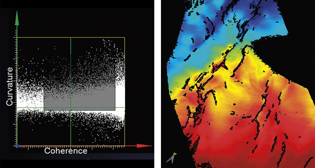
Cross-plotting provides a means of separating different types of faults. Faults that have significant drag may appear in both coherence and most-positive and most-negative curvature images. However faults that do not have drag will often not appear on curvature. Very subtle faults exhibiting subseismic wavelet offset often do not appear in coherence. Crossplotting is an iteractive means of clustering such differences. It may be noted that the attribute volumes (coherence and curvature) used for cross-plotting, should be free from noise as much as possible. Acquisition footprint may easily fall in the top-left quadrant used for polygon-connect and interfere with meaningful analysis. For this purpose, we recommend conditioning of the seismic data going into attribute computation through the application of structure-oriented filtering (PC or Principal- Component Filtering) (Chopra and Marfurt, 2008).

Calibration with well log data

If possible, it is always a good idea to calibrate the interpretation on curvature displays with log data. One promising way is to interpret the lineaments in a fractured zone and then transform them into a rose diagram. Such rose diagrams can then be compared with similar rose diagrams that are obtained from image logs to gain confidence in the seismic-to-well calibration. Once a favorable match is obtained, the interpretation of fault/fracture orientations and the thicknesses over which they extend can be used with greater confidence for more quantitative reservoir analysis. Needless to mention such calibrations need to be carried out in localized areas around the wells for accurate comparisons.

Rose diagrams

Fractures are characterized by lineaments that are oriented in different directions. Rather than view individual lineament orientation at a given point, it is possible to combine the various orientations in all directions into a single rose diagram with angles ranging from 1 to 180 degrees. The length of each petal of the rose is dependent on the frequency of lineaments falling along any angle. Rose diagrams are commonly used for depicting orientations of specific lineaments and are preferred due to their ease of comprehension (Wells, 2000).

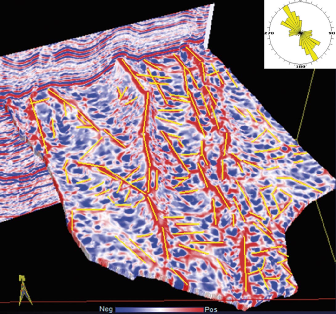
Figure 9 shows lineaments picked up on the most-positive curvature display in yellow-colored line segments. These are then transformed into a rose diagram shown in the inset. Notice, in one single display it is possible to see the orientation of fractures and their density on this surface. Strictly speaking, this rose diagram should be generated at a localized area around a given borehole, instead of over the whole area of the seismic volume.

3D rose diagrams

The curvedness of a surface is calculated as c²= k_min² + k_max².

where k_min and k_max are the minimum and maximum curvature (Roberts, 2001). Roberts (2001) also shows how k_min and k_max can be used to compute a shape index, s, which defines dome (s=+1), ridge (s=+1/2), saddle (s=0), valley (s=-1/2), and bowl (s=-1) quadratic surfaces. The curvedness defines the intensity of deformation in generating these shapes, with a planar surface being defined as c=0.

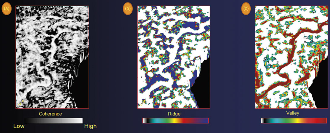
Al-Dossary and Marfurt (2006) showed how the intensity of deformation can be combined with the shape index to generate shape components, with the sum of the components equal to the curvedness. The choice of shape depends on the geological model being used. In Figure 10 we show a comparison of the coherence horizon slice with the valley and the ridge horizon slices. Note that the edges of the channel are accentuated by the ridge attribute and the thalweg of the channel is defined better by the valley attribute. Ridges and valleys (as well as elongated domes and bowls) have a well-defined strike. We will therefore interpret the azimuth of minimum curvature, ψ_min, to be a direct measurement of the strike of ridges and valleys.

For a more conventional display and qualification of lineaments, we generate rose diagrams for any gridded-square area containing n-inline by m-crossline analysis window, for each horizontal time slice. Within each analysis window, we bin each pixel into rose petals according to its azimuth ψ_min in, weighted by its threshold-clipped ridge or valley components of curvedness, then sum and scale them into rose diagrams. The process is repeated for the whole data volume. After that, the rose diagrams are mapped to a rose volume which is equivalent to the data volume, and centered in the analysis window, located at the same location as in input data volume. A robust generation of rose diagrams for the whole lineament volume (corresponding to seismic volume) is completed, yielding intensity and orientation of lineaments.

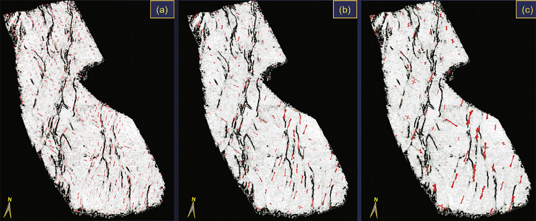
In this manner, we generate 3D rose diagrams from either the ridge or valley component of curvature and the azimuth of minimum curvature. The choice of ridge or valley depends on the geological processes that formed them. Thus, if we wish to generate rose diagrams of a channel-levee system, rose diagrams generated from valley component of curvature would be a direct measure of the channel axes. Likewise, the valley component of curvature is a direct measure of intensity of karst-enhanced fractures in an otherwise planar carbonate horizon. Thus 3D rose diagrams are generated from two significant attributes namely the azimuth of minimum curvature and as stated above another attribute that would have a good measure of the shape of the features. This attribute could be the valley attribute or the ridge attribute. Figure 11 shows the generation of the rose diagrams from the ridge component of curvature, as well as the azimuth of the minimum curvature attribute. Notice, the displays seems to correlate well in that the lineaments seen on coherence seem to align well with the rose petals, and where there are no lineaments seen on the coherence display, the rose petals do not exhibit significant size. As the size and lateral spacing of rose generation can be controlled, an optimum spread of the roses needs to be ascertained. To do so, in Figure 11 we also show the roses generated at a specific choice of the search radius. Apparently, the roses with a radius of 600m appear to have their spread reasonably matching the lineaments seen matching the lineaments on the coherence.

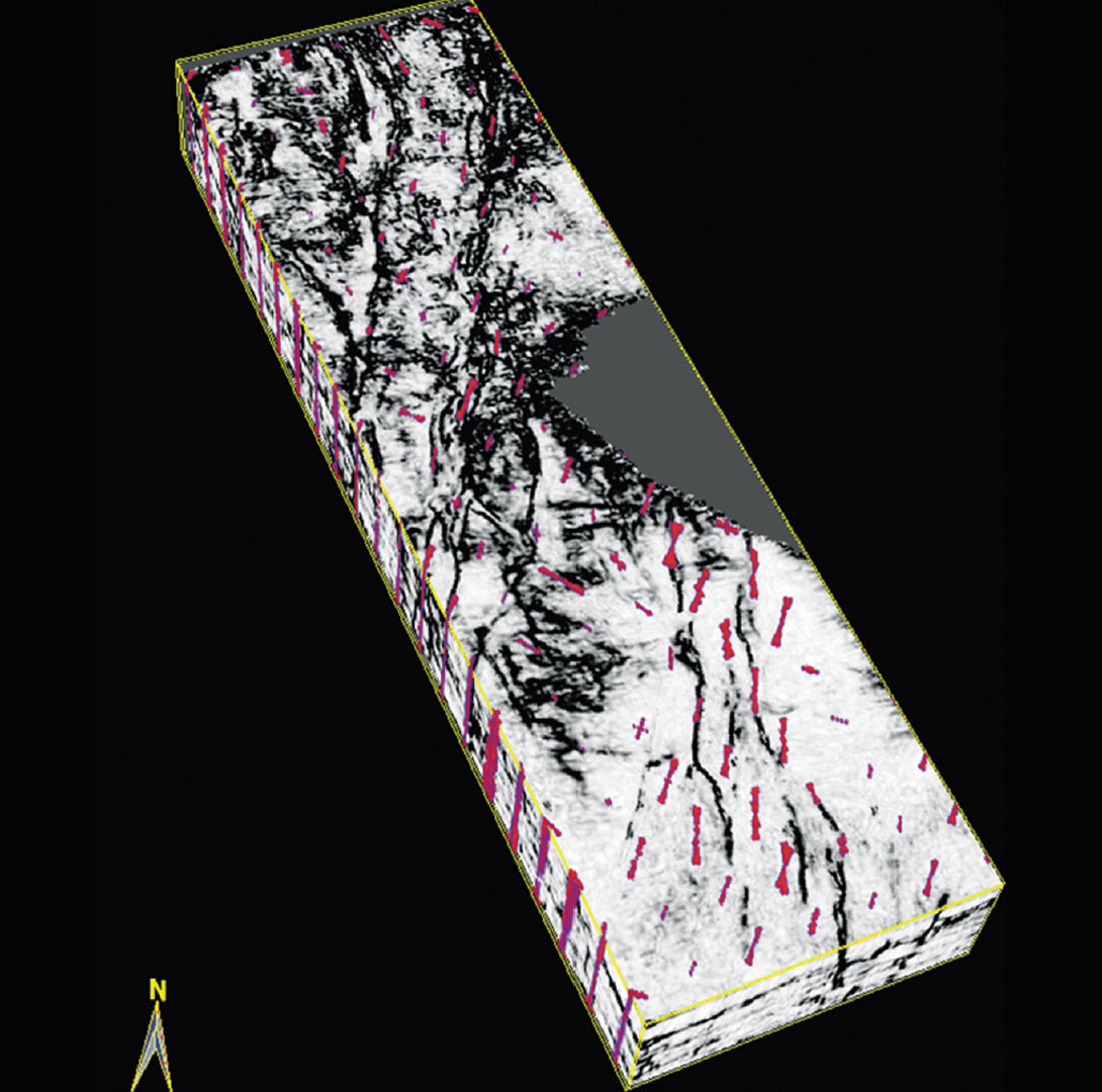
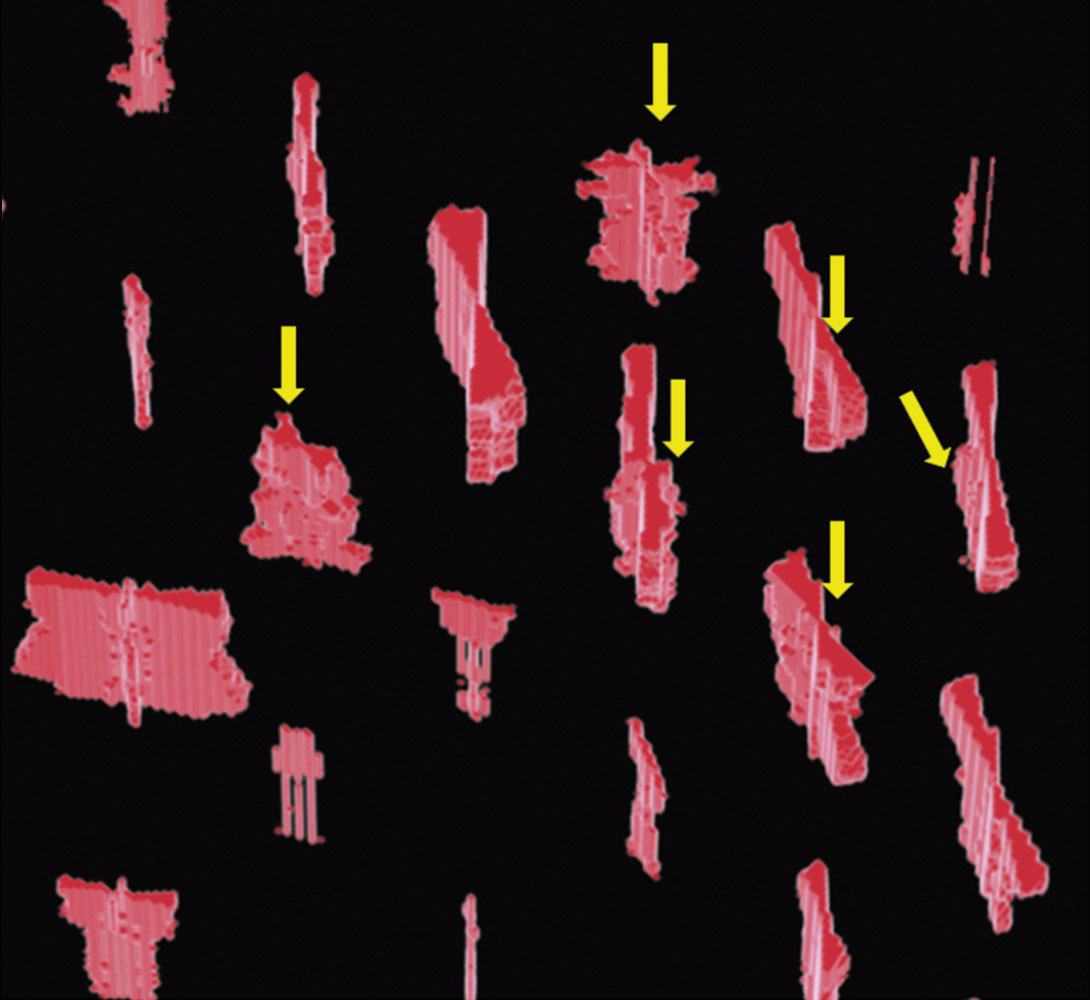
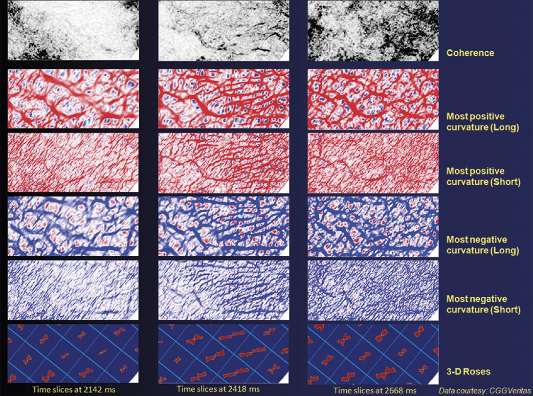
As shown in the foregoing examples, a significant advantage of the volumetric generation of roses at grid nodes is that it is possible to merge them with a suitable attribute volume. Figure 12 shows the merge of a stratal volume from coherence with the rose volume. It is possible to animate through this volume to the desired level and then examine how the lineaments match the rose petals. A blowup of the rose diagram volume is shown in Figure 13. Such 3D roses help the interpreter notice, within the thickness of the strat-cube shown, whether the orientation of the fractures remains the same or changes. There are at least five roses marked with arrows that indicate changes in orientation of fractures with depth. This point is illustrated very nicely in Figure 14, where we show a comparison of different coherence and curvature (both positive and negative as well as long and short wavelength) time slices, as well as 3D rose diagram displays. Notice, at 2142 ms the fractures have an orientation that is almost NESW. However, at 2418 ms not only does the orientation change close to E-W, but the density of fractures also increases. At 2668 ms the orientation is again NE-SW.

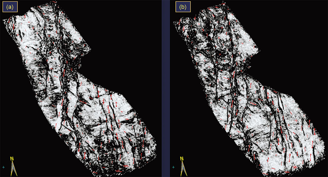
Finally, another advantage of such a composite visualization is that in multi-level fracture zones of interest, it is possible to animate to these desired fracture zones. Figure 15 shows strat-slices at 50 ms and 100 ms below a marker horizon. Notice how nicely the petal orientations match the low coherence lineaments seen on these displays.

Conclusions

Seismic discontinuity attributes can be a great help in characterizing fractures. We have described various ways in which it is possible to describe the presence, density, and orientation of fractures. Coherence and curvature are useful attributes that an interpreter can use for the purpose. Volume visualization of stratigraphic features and fractures and in particular, is a great aid in 3D seismic interpretation, and the right way to get the true perspective of subsurface features. Interpretation of the stratigraphic subsurface features can be greatly aided by adopting cross-plotting of seismic discontinuity attributes in the interpretation workflow as we have demonstrated here. This would save the seismic interpreters considerable time and effort in going through the laborious task of carrying out interpretation on individual profiles in the 3D volume. The saved time could be used more fruitfully in addressing critical prospect issues.

3D rose diagrams can be generated as a volume using either the ridge or the valley shape attribute in combination with the azimuth of minimum curvature attribute. Such a volume can be merged with any other attribute volume that has been generated to study the fracture lineaments and their orientation. We have illustrated this application through examples from real seismic data volumes from Alberta, Canada. Visualization of these volumetric 3D rose diagrams with other discontinuity attributes lends confidence to the interpretation of fracture lineaments. Finally, such 3D rose diagrams can be correlated with similar rose diagrams from image logs.

Acknowledgements

I would like to thank Fairborne Energy, Kuwait Oil Company, POGC, FX Energy, and Tanganyika Oil Company for permission to show some of the examples in the presentation. I would like to thank CGGVeritas Data Library, Calgary for permission to show examples from Fairborne Energy, and Geomodeling Technology Corporation, Calgary for help with the operations of their software used for generating displays shown in this work. Finally, I also wish to thank Arcis Corporation for the support in the development of this work, the data examples to be shown and permission to publish this work.