Interesting pursuits in seismic curvature attribute analysis

Summary

Since they are second-order derivatives, seismic curvature attributes can enhance subtle information that may be difficult to see using first-order derivatives such as the dip magnitude and the dip-azimuth attributes. As a result, these attributes form an integral part of most seismic interpretation projects. In this article we discuss some of the recent developments in curvature attributes that we have been pursuing. These are the computation of amplitude curvature attribute and its comparison with the conventional structural curvature attribute, Euler curvature which is also termed as azimuthal curvature, and the seismic reflection rotation and vector convergence attributes.

The conventional computation of curvature may be termed as structural curvature, as lateral second-order derivatives of structural component of seismic time or depth of reflection events are used to generate them. Here, we explore the case of applying lateral second-order derivatives on the amplitudes of seismic data along the reflectors. We refer to this second computation as amplitude curvature. For volumetric structural curvature we compute first-derivatives of the volumetric inline and crossline components of structural dip. For amplitude curvature we apply a similar computation to the volumetric inline and crossline components of the energyweighted amplitude gradients, which represent the directional measures of amplitude variability. Since the amplitude and structural position of a reflector are mathematically independent properties, application of amplitude curvature computation to real seismic data often shows different, and sometimes more detailed illumination of geologic features than structural curvature. However, many features, such as the delineation of a fault where we encounter both a vertical shift in reflector position and a lateral change in amplitude, will be imaged by both attributes, with images ‘coupled’ through the underlying geology.

Euler curvature is a generalization of the dip and strike components of curvature in any user-defined direction, and may be called azimuthal curvature or more simply apparent curvature (similar to apparent dip). Euler curvature is useful for the interpretation of lineament features in desired azimuthal directions, say, perpendicular to the minimum horizontal stress. If a given azimuth is known or hypothesized to be correlated with open fractures or if a given azimuth can be correlated to enhanced production or effective horizontal drilling, an Euler-curvature intensity volume can be generated for that azimuth thereby high-grading potential sweet spots.

Geometric attributes such as coherence and curvature are useful for delineating a subset of seismic stratigraphic features such as shale dewatering polygons, injectites, collapse features, mass transport complexes and overbank deposits, but have limited value in imaging classic seismic stratigraphy features such as onlap, progradation and erosional truncation. In this context, we review the success of current geometric attribute usage and discuss the applications of newer volumetric attributes such as reflector convergence and reflector rotation about the normal to the reflector dip. While the former attribute is useful in the interpretation of angular unconformities, the latter attribute determines the rotation of fault blocks across discontinuities such as wrench faults. Such attributes can facilitate and quantify the use of seismic stratigraphic workflows to large 3D seismic volumes.

Structural curvature versus amplitude curvature

Since the introduction of the seismic curvature attributes by Roberts (2001), curvature has gradually become popular with interpreters, and has found its way into most commercial software packages. Curvature is a 2D second-order derivative of time or depth structure, or a 2D first-order derivative of inline and crossline dip components. As a derivative of dip components, curvature measures subtle lateral and vertical changes in dip that are often overpowered by stronger, regional deformation, such that a carbonate reef on a 20° dipping surface gives rise to the same curvature anomaly as a carbonate reef on a flat surface. Such rotational invariance provides a powerful analysis tool that does not require first picking and flattening on horizons near the zone of interest. Curvature computation can be carried out on both time surfaces as well as 3D seismic volumes. Roberts (2001) introduced curvature as a 2D second-derivative computations of picked seismic surfaces. Soon afterwards, Al-Dossary and Marfurt (2006) showed how such computations can be computed from volumetric estimates of inline and crossline dip components. By first estimating the volumetric reflector dip and azimuth that best represents each single sample in the volume, followed by computation of curvature from adjacent measures of dip and azimuth, a full 3D volume of curvature values is produced.

To clarify our subsequent discussion, we denote the above calculations as structural curvature, the (explicit or implicit) lateral second derivatives of reflector time or depth. Many processing geophysicists focused on statics and velocity analysis think of seismic data as composed of amplitude and phase components, where the phase associated with any time t and frequency f is simply φ=2πft. Indeed, several workers have used the lateral change in phase as a means to compute reflector dip (e.g. Barnes, 2000; Marfurt and Kirlin, 2000).

We can also compute second derivatives of amplitude. Horizon-based amplitude curvature is in the hands of most interpreters. First, we generate a horizon slice through a seismic amplitude, RMS amplitude, or impedance volume. Next, we compute the inline (∂a /∂x) and crossline (∂a /∂y) derivatives of this map. Such maps can often delineate the edges of bright spots, channels, and other stratigraphic features at any desired direction, θ, by combining the two measures with simple trigonometry (cosθ∂a /∂x+sinθ∂a /∂y). A common edge detection algorithm is to compute the Laplacian of a map (though more of us have probably applied this filter to digital photographs than to seismic data),

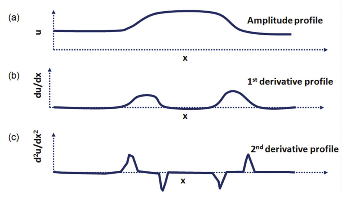
Equation 1 is the formula for the mean amplitude curvature. In Figure 1 we show a schematic diagram of an amplitude anomaly exhibiting its lateral change in one direction, x. Thereafter, we compute the 1st and 2nd spatial derivatives of the amplitude with respect to x and show the results in Figure 1b and c. Notice, the extrema seen in Figure 1c demarcate the limits of the anomaly.

Luo et al. (1996) showed that if one were to first estimate structural inline and crossline dip, then one can generate an excellent edge detector that is approximately

where the derivatives are computed in a (-K to +K vertical sample, J-trace) analysis window oriented along the dipping plane and the derivatives are evaluated at the center of the window. Marfurt and Kirlin (2000) and Marfurt (2006) showed how one can compute accurate estimates of reflector amplitude gradients, g, from the KL-filtered (or principal component of the data) within an analysis window:

where v₁ is the principal component or eigenmap of the J-trace analysis window, and λ₁ is its corresponding eigenvalue, which represents the energy of this data component.

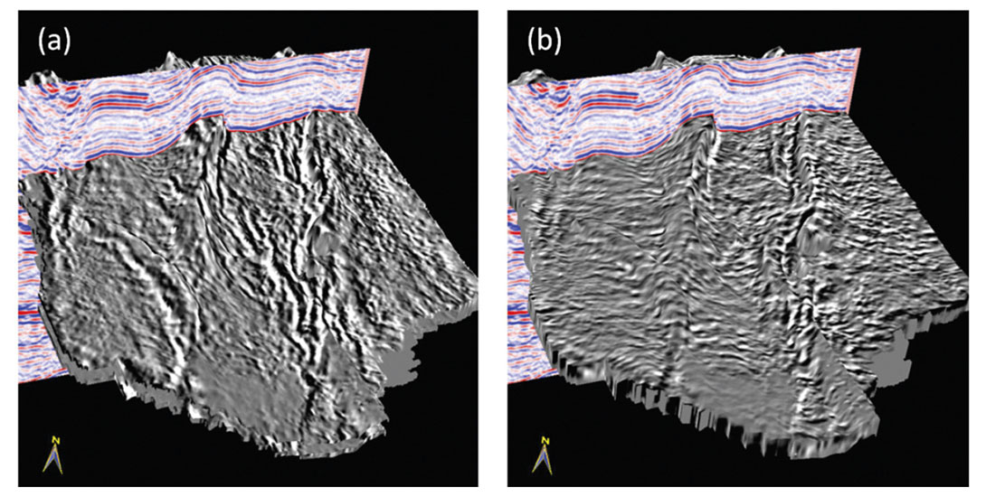
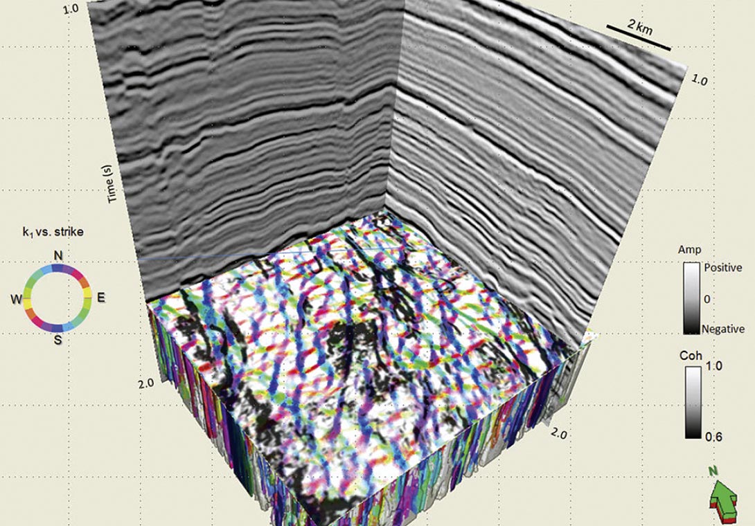
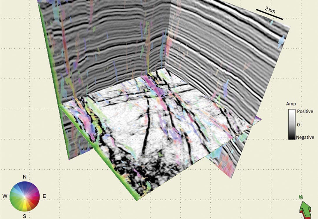
In Figures 2a and b we show the images for 3D chair views wherein the vertical section is the seismic inline and is seen being correlated with the energy-weighted amplitude gradient in the inline and the crossline gradients respectively. Both images express independent views of the same geology (almost N-S oriented main faults and fault related fractures) much as two orthogonal shaded illumination maps.

For volume computation of structural curvature, the equations applied to the components of reflector dip and azimuth in the inline and crossline directions are given by Al-Dossary and Marfurt (2006). In the case of amplitude computation of curvature, nearly the same equations are applied to the inline and crossline components of energy-weighted amplitude gradients which represent the directional measures of amplitude variability.

Geological structures often exhibit curvature of different wavelengths and so curvature images of different wavelengths provide different perspectives of the same geology. Al-Dossary and Marfurt (2006) introduced the volume computation of longand short-wavelength curvature measures from seismic data. Many applications of such multispectral estimates of curvature from seismic data have been demonstrated by Chopra and Marfurt (2006, 2007a and b, 2010). Short wavelength curvature often delineates details with intense highly localized fracture systems. Long wavelength curvature on the other hand enhances subtle flexures on a scale of 100-200 traces that are difficult to see on conventional seismic data, but are often correlated to fracture zones that are below seismic resolution as well as to collapse features and diagenetic alterations that result in broader bowls.

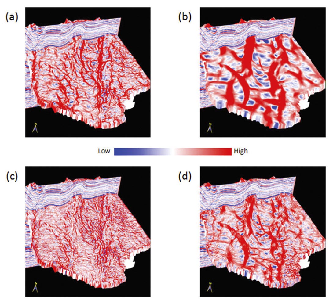
In Figures 3 and 4 we show a comparison of the long- and short-wavelength computation of most-positive and most-negative amplitude and structural curvature measures. In Figure 3 we notice that for both long and short wavelength, the amplitude curvature estimates provide additional information. Structural most-positive curvature displays in Figure 3b and d show lower frequency detail as compared with their equivalent amplitude curvature displays in Figures 3a and c. Similarly, Figures 4 a and c exhibit much greater lineament detail on the amplitude most-negative curvature displays than what is seen on structural most-negative curvature displays in Figure 4b and d. Such fine detail is very useful when using curvature attributes for fault /fracture delineation, particularly those that give rise to measureable amplitude changes but minimal changes in dip, such as cleats in coal beds. In Figures 5 and 6 we show a similar comparison where again we observe higher level of lineament detail on both long and short-wavelength amplitude curvature in preference to structural curvature.

Euler curvature

In his seminal paper Roberts (2001) describes twelve different types of surface-based attribute measures. Many of these attributes have been extended to volume computations and implemented on interpretation workstations. Of these different curvature attributes, the most-positive and the most-negative principal curvatures k₁ and k₂ are the most popular. Not only are k₁ and k₂ intuitively easy to understand, they also provide more continuous maps of faults and flexures than the maximum and minimum curvatures, k_max and k_min, which can rapidly change sign at fault and flexure intersections. While other attributes such as the mean curvature, Gaussian curvature and shape index have also been used by a few practitioners, there are some other curvature attributes which Roberts (2001) introduced that warrant investigation and forms the motivation for the present work.

Definition and workflow

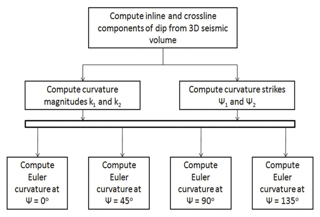
In this paper, we describe the application of volumetric Euler curvature to 3D seismic data volumes. Euler curvature can be thought of as apparent curvature along a given strike direction. If (k₁ , ψ₁) and (k₂ , ψ₂) represent the magnitude and strike of the most-positive and most-negative principal curvatures then the Euler curvature at an angle ψ in the dipping plane tangent to the analysis point (where ψ₁ and ψ₂ are orthogonal) is given as

Since reflector dip magnitude and azimuth can vary considerably across a seismic survey, it is more useful to equally sample azimuths of Euler curvature on the horizontal x-y plane, project these lines onto the local dipping plane of the reflector, and implement equation 4. The flow diagram in Figure 7 explains the method for computing Euler curvature.

Applications

Mapping the intensity of a given fracture set has been a major objective of reflection seismologists. The most successful work has been using attributes computed by azimuthally-limited prestack data volumes. Chopra et al. (2000) showed how coherence attributes computed from azimuthally-restricted seismic volumes can enhance subtle features hidden or blurred in the all-azimuth volume. Vector-tile and other migration-sorting techniques are now the method of choice for both conventional Pwave and converted wave prestack imaging (e.g. Jianming et al., 2009) allowing one to predict both fracture strike and intensity.

Curvature, acoustic impedance, and coherence are currently the most effective attributes used to predict fractures in the post-stack world (e.g. Hunt et al., 2010). Rather than map the intensity of the strongest attribute lineaments, Singh et al. (2008) used an image-processing (ant-tracking) algorithm to enhance curvature and coherence lineaments that were parallel to the strike of open fractures, at an angle of some 45° to the strike of the strongest lineaments. Henning et al. (2010) use related technology to azimuthally filter lineaments in the Eagleford formation of south Texas. They then compute RMS maps of each azimuthally-limited volume that can be correlated to production. Guo et al. (2010) hypothesize that each azimuthally-limited attribute volume computed from k₁ and ψ₁ corresponds to open fractures. Each of these volumes is then correlated to production to either validate or reject the hypothesis.

Daber and Boe (2010) described the use of what they referred to as azimuthal curvature (and is described here as Euler curvature following Roberts (2001) definition) for reducing noise in poststack curvature volume. They show that if the azimuthal direction is set to the inline, then the curvature computation would ignore the crossline directions and this would reduce the acquisition noise.

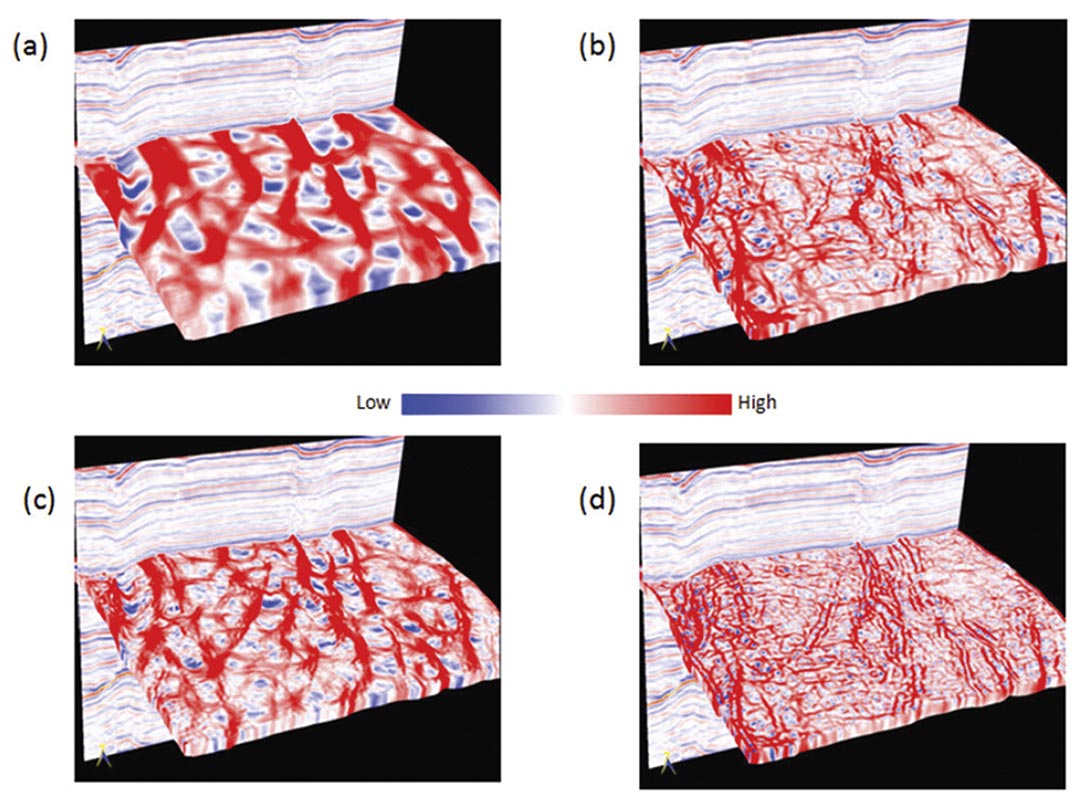
We describe here the application of Euler curvature to two different 3D seismic volumes from northeast British Columbia, Canada. We propose an interactive workflow, much as we do in generating a suite of shaded relief maps where we display apparent dip rather than apparent (Euler) curvature. In Figure 8 we show 3D chair view displays for Euler curvature run at 0°, 45°, 90° and 135°. The left column of displays shows the long-wavelength version and the right display the short wavelength displays. Notice for 00 azimuth (which would be the north), lineaments in the E-W direction seem to stand out. For 45°s, the lineaments that are almost NW-SE are seen pronounced. Similarly for 90°s the roughly N-S events stand out and for 135°s the events slightly inclined to the vertical are more well-defined.

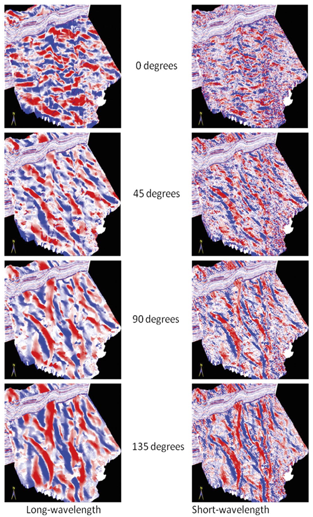
The same description applies to the short-wavelength displays that show more lineament detail and resolution than the long-wavelength display.

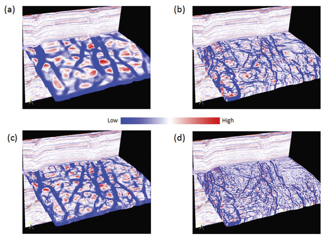
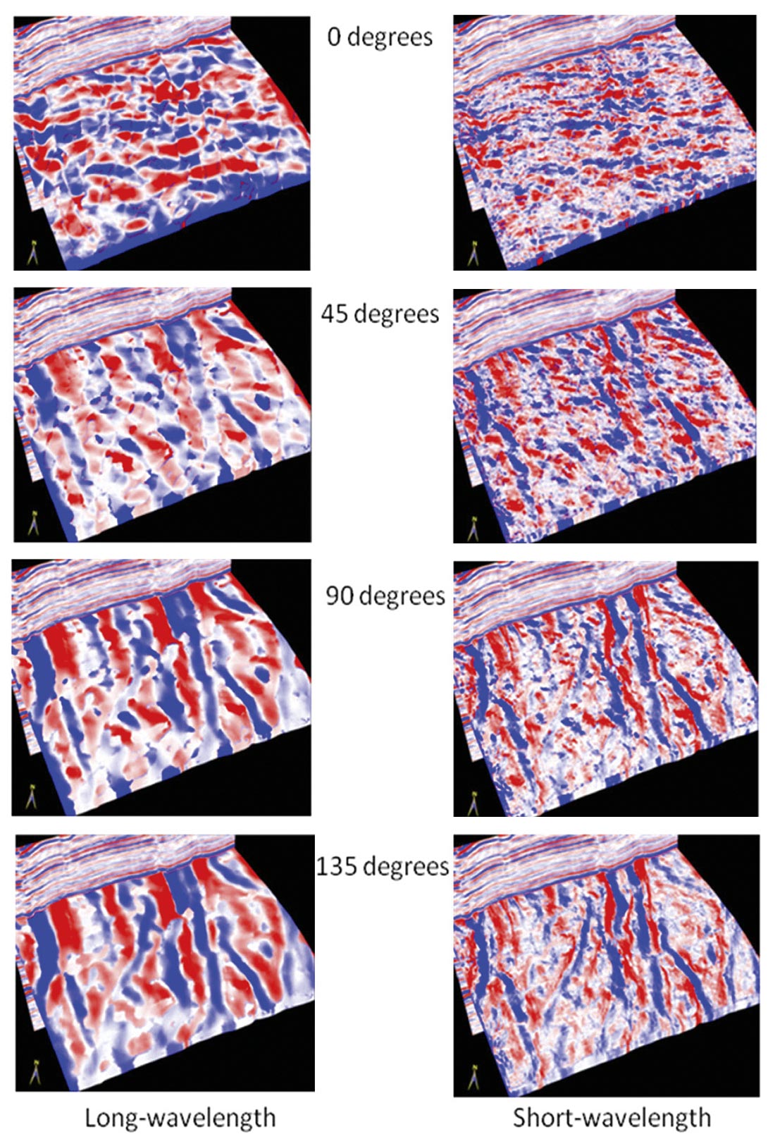
In Figure 9 we show a similar 3D chair view displays and again notice the lineaments becoming pronounced for particular azimuth directions.

There are obvious advantages to running Euler curvature on post stack seismic volumes in that the azimuth directions can be carefully chosen to highlight the lineaments in the directions known through image logs or production data to better correlate to open fractures. This does not entail the processing of azimuth-restricted volumes (usually three or four) all the way to migration and then passing them through coherence/curvature computation.

Volumetric estimates of seismic reflector rotation and convergence

Seismic stratigraphic analysis refers to the analysis of the configuration and termination of seismic reflection events, packages of which are then interpreted as stratigraphic patterns. These packages are then correlated to well-known patterns such as toplap, onlap, downlap, erosional truncation, and so forth, which in turn provide architectural elements of a depositional environment (Mitchum et al., 1977). Through well control as well as modern and paleo analogues, we can then produce a probability map of lithofacies.

Geometric attributes such as coherence and curvature are commonly used for mapping structural deformation and depositional environment. Coherence proves useful for identification of faults, channel edges, reef edges and collapse features while curvature images folds, flexures, sub-seismic conjugate faults that appear as drag or folds adjacent to faults, roll-over anticlines, diagenetically altered fractures, karst and differential compaction over channels.

Although coherence and curvature are excellent at delineating a subset of seismic stratigraphic features (such as shale-dewatering polygons, injectites, collapse features, mass transport complexes, and overbank deposits) they have only limited value in imaging classic seismic stratigraphy features such as onlap, progradation and erosional truncation. We review the success of current geometric attribute usage and examine how the newer volumetric attributes can facilitate and quantify the use of seismic stratigraphic analysis workflows to large 3D seismic volumes.

Attribute application for stratigraphic analysis

Due to the distinct change in reflector dip and/or terminations, erosional unconformities and in particular angular unconformities are relatively easy to recognize on vertical seismic sections. Although there will often be a low-coherence anomaly where reflectors of conflicting dip intersect, these anomalies take considerable skill to interpret. Barnes (2000) was perhaps the first to discuss the application of attributes based on the description of seismic reflection pattern and used them to map angular unconformities amongst other features. As the first step volumetric estimates for vector dip are computed. Next, the mean and standard deviation of the vector dip are calculated in narrow windows. Those reflections that exhibit parallelism have a smaller standard deviation and while non-parallel events such as angular unconformities have a higher standard deviation.

Computing a vertical derivative of apparent dip at user-defined azimuth, Barnes (2000) defined the convergence/divergence of reflections. Convergent reflections would show a decreasing dip with depth/time at constant azimuth. Marfurt and Rich (2010) built upon Barnes’ (2000) method by taking the curl of the volumetric vector dip thereby generating a 3D reflector convergence azimuth and magnitude estimates.

Compressive deformation and wrench faulting cause the fault blocks to rotate (Kim et al., 2004). Such rotation has been observed in laboratory measurements. The extent of rotation depends on the size, the comprising lithology and the stress levels. As the individual fault blocks undergo rotation, it is expected that the edges experience higher stresses and undergo fracturing.

Natural fractures are controlled by fault block rotation and depend on how the individual fault segments intersect. Fault block rotation can also control depositional processes by providing increased accommodation space in subsiding areas and erosional processes in uplifted areas. In view of this importance of the rotation of the fault blocks, a seismic attribute application focusing on the rotation of the fault blocks is required. Besides the reflector convergence attribute mentioned above, Marfurt and Rich (2010) also discuss the calculation of another attribute that determines the rotation about the normal to the reflector dip and would be a measure of the reflector rotation across a discontinuity such as a wrench fault.

As the first step, the inline and crossline components of dip are determined at every single sample in the 3D volume using semblance search or any other available method. After defining the three components of the unit normal, n, and the rotation vector ψ, Marfurt and Rich (2010) define the rotation about the normal to the reflector dip as

which is essentially a measure of the reflector rotation across a discontinuity such as a wrench fault.

Similarly, Marfurt and Rich (2010) write reflector convergence as follows:

Examples

Note that the reflector convergence, c, is a vector consisting of a magnitude and azimuth. We use a common 2D color wheel to display such a result, where parallel reflectors (magnitude of convergence = 0) appear as white, and the azimuth of convergence is mapped against a cyclical color bar, with the colors becoming darker for stronger convergence. In Figure 10, we try and explain the convergence within a channel with or without levee/overbank deposits, in terms of the following cases:

Case-1: where the deposition within the channel shows no significant convergence;

Case-2: where the deposition within the channel is such that the west channel margin is converging towards the west and the east channel margin is converging towards the east. This is displayed in color to the right with the help of a 2D color wheel;

Case-3: where the deposited sediments within the channel are not converging at the margins, but the levee/overbank deposits converge towards the channel (west deposits converge towards the east and vice-versa;

Case-4: where both the strata within the channel and levee/overbank deposits are converging. This appears to be a combination of cases 2 and 3 above.

Notice how the convergence shows up in color (using the 2D color wheel) as displayed to the right in cyan and magenta colors along the channel edges.

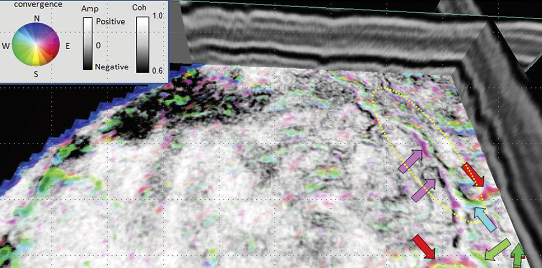
We carried out the computation of reflector convergence and the rotation about the normal to the reflector dip attributes for a suite of 3D seismic volumes from Alberta, Canada. Figure 11 depicts a 3D chair view with a coherence time slice exhibiting a channel system, co-rendered with reflector convergence attribute using a 2D color wheel. Within the area highlighted by the ellipse in yellow dotted line, an interpretation has been made keeping in mind the cases shown in Figure 10. Apparently, the levee/overbank deposit converging towards the channel margin generating the magenta and green colors with respect to the reflector convergence.

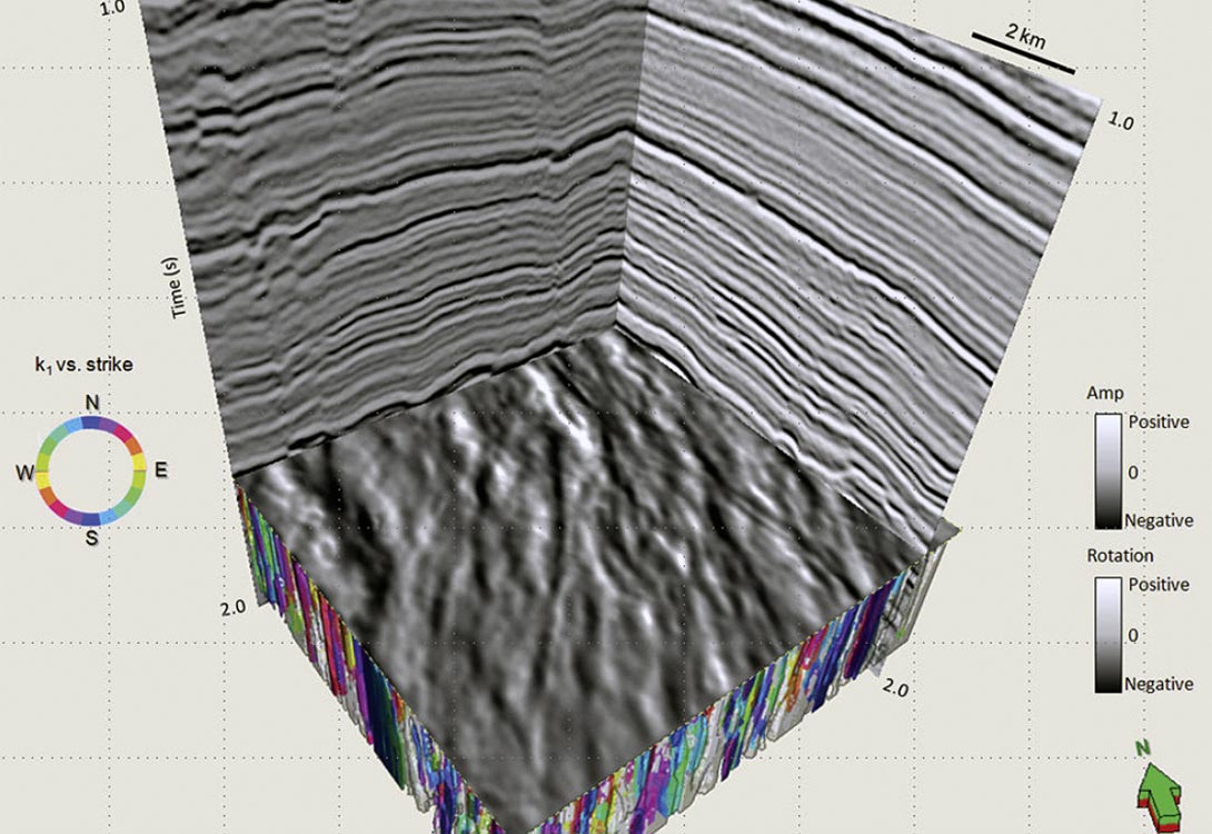
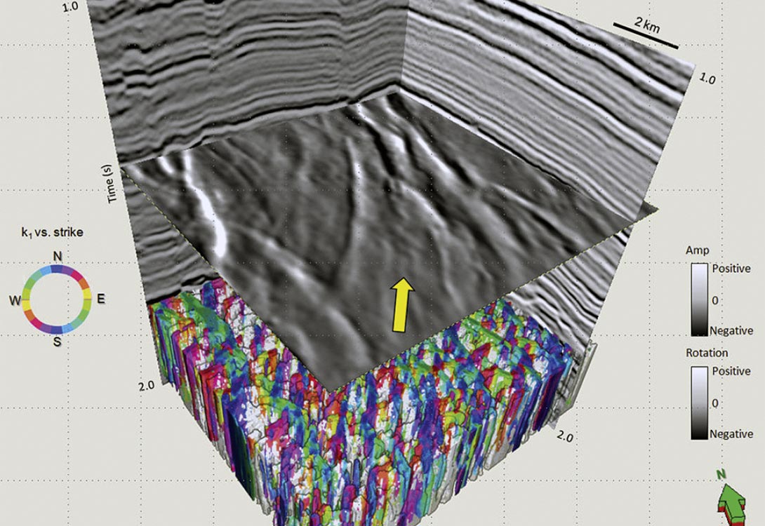
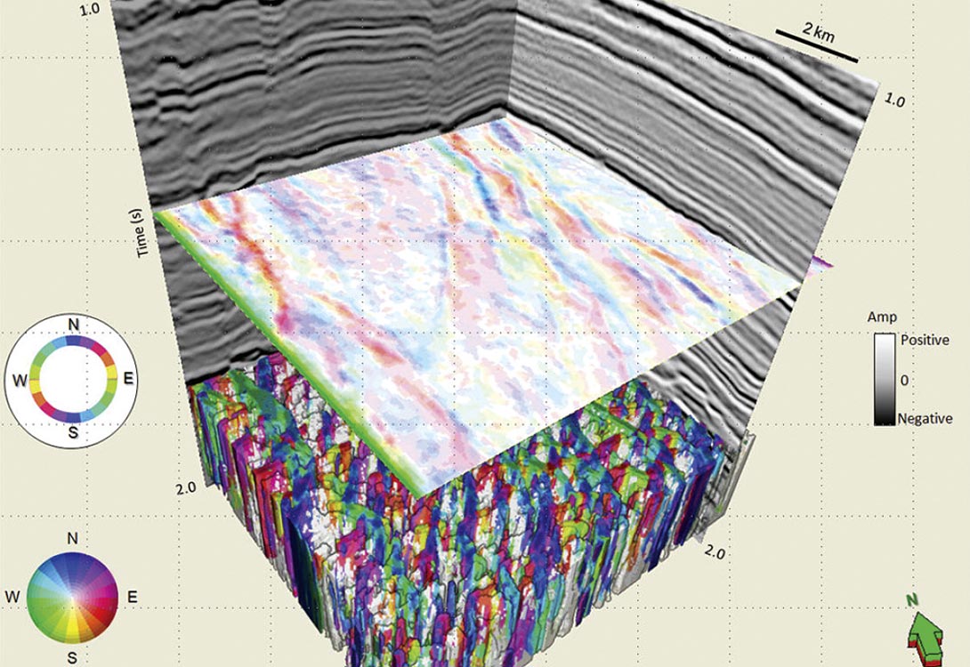
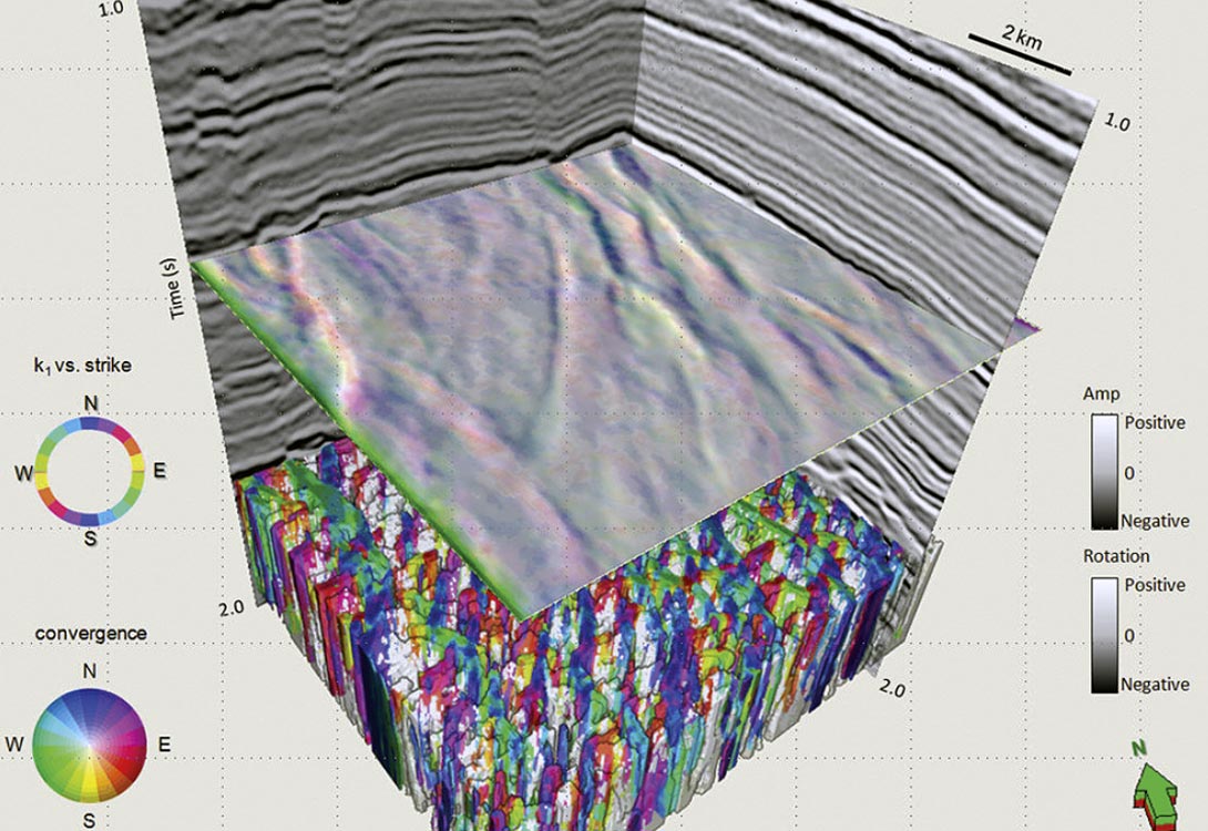
In Figure 12, we show a 3D chair display with the vertical inline and crossline displays and a time slice at 1.710 s from a coherence volume showing several lineaments corresponding to faults associated with a network of horst and grabens. This time slice is co-rendered with a multiattribute volume of the strike of the most-positive principal curvature, ψ₁, (plotted against hue) modulated by the magnitude of the most positive principal curvature, k₁. The fault blocks give rise to prominent North- South trending lineaments (depicted as blue) as well NE-SW trending faults (red) and NW-SE trending faults (cyan and green). In Figure 13 we show a corresponding time slice through the reflector rotation about the average reflector normal volume. Notice the horst and graben features show considerable contrast so as to be conveniently interpreted. Again in Figure 14 which shows a similar display, the time slice is at 1.330 s from the reflector rotation attribute about the average reflector normal. The yellow arrow is indicative of either a rotation about antithetic faults or a suite of relay ramps. An equivalent display is shown in Figure 15, but with the time slice from the reflector convergence attribute. The display uses a 2D color wheel (shown in Figure 10), wherein the blue color indicates reflectors pinching out to the North, red to the Southeast and cyan to the Northwest. We co-render the slices in Figures 14 and 15 using 50 percent transparency and obtain a display as shown in Figure 16. The thickening and thinning of the reflectors appear to be controlled by rotating fault blocks.

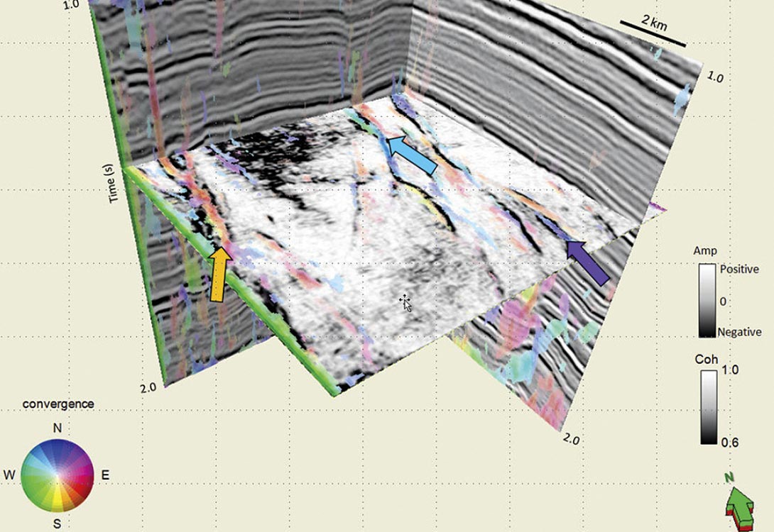
In Figure 17 we see a time slice at 1.330 s through the coherence attribute in gray scale co-rendered with the reflector convergence displayed against a 2D color wheel. The orange arrow indicates sediments in the graben thinning to the Southeast. The sediments indicated by the cyan arrow show thinning to the Northwest and by the purple arrow to the North-Northeast. Sediments that have low convergence magnitude or which are nearly parallel, has been rendered transparent. A similar display we show in Figure 18 with the time slice at 1.550s.

Conclusions

1. For data processed with an amplitude preserving sequence, amplitude variations are diagnostic of geologic information such as changes in porosity, thickness and /or lithology. Computation of curvature on amplitude gradients furnishes higher level of lineament information that appears to be promising. The application of amplitude curvature to impedance images is particularly interesting (Guo et al., 2010). We hope to extend this work to the generation of rose diagrams for the lineaments observed on amplitude curvature and make comparisons with similar roses obtained from image logs. Such exercises will lend confidence in the application of amplitude curvature in seismic data interpretation.
2. Euler curvature run in desired azimuthal directions exhibit a more well-defined set of lineaments that may be of interest. Depending on the desired level of detail, the longor the short-wavelength computations can be resorted to. For observing fracture lineaments the short-wavelength Euler curvature would be more beneficial. This work is in progress and we hope to calibrate the observed lineaments with the image logs in terms of rose diagram matching. This would serve to enhance the interpreter’s level of confidence, should the rose-diagrams match.
3. As shown above, application of two attributes, namely reflector convergence and the rotation about the normal to the reflector dip are shown on two different 3D seismic volumes from Alberta, Canada. These attributes have both been found to be very useful. Reflector convergence attribute gives the magnitude and direction of thickening and thinning of reflections on uninterpreted seismic volumes. Reflector rotation about faults is clearly evident and has a valuable application in mapping of wrench faults. Such attributes would yield convincing results on datasets that have good quality. Dip-convergence based attributes do not delineate disconformities and nonconformities exhibiting near parallel reflector patterns. Condensed sections are often seen as stratigraphically parallel low-coherence anomalies on vertical sections. More promising solutions to mapping these features are based on changes in spectral magnitude components (Smythe et al., 2004) or in spectral phase components (Castro de Matos et al., 2011).