Geologically Reasonable Vεδθ Models for Depth Imaging

Introduction

“The interpretation of observed elastic wave velocities in the rocks of the earth’s crust is our principal basis for inferring its structure at inaccessible depths.” Ide, 1936.

Ide’s statement is as true today as it was back in 1936. He goes on to talk about the practical nature of geophysics and how the observed time differences are more important than the actual velocities in different rocks. This is no longer true. With the advent of depth imaging, there is a paradigm shift back to requiring the actual velocities of elastic waves travelling through rock.

In recent years the focus of seismic processing has moved from time imaging to depth imaging. Time imaging is often preferred for its simplicity in determining imaging velocities to create an image of the subsurface. However, in areas of complex deformation, that contain laterally varying velocity fields, depth migration is required. Instead of imaging velocities, depth migration uses smoothed interval velocities. Determining interval velocities for depth processing is challenging but provides additional information regarding the subsurface. Time migration is less sensitive than depth migration to variations in the velocity model, but may distort structures in areas with lateral velocity variations and introduces the possibility of interpretation pitfalls. These pitfalls may often be eliminated with the use of a precise velocity model to convert time sections to depth sections, although this will not resolve the lateral mis-positioning of structures in time-migrated sections.

In the case of complex structures with steep dips, lateral velocity changes and closely spaced folds and faults, depth migration is necessary to correctly position reflectors. However, to obtain the correct image we ultimately require the correct velocity model. In addition, anisotropy further confounds the issue and, if ignored, leads to greater errors in the final image and therefore must also be included in the velocity model.

In the case of isotropic prestack depth migration, velocity is independent of the wave propagation direction, and therefore, only a scalar velocity value is required for each subsurface location. Despite the long term success of the isotropic assumption, the Earth may be, in fact, anisotropic and, if so, should be treated as such in seismic imaging. Many studies have shown that transverse isotropy, a form of anisotropy, sufficiently characterises wave propagation through clastic strata, in which case, four parameters are required to fully characterise P-wave propagation. When Thomsen’s (1986) parameters of anisotropy are utilised, a four-parameter model is required to undertake the migration, namely (V₀, ε, δ and θ), that we refer to as the ‘Vεδθ’ model, where V represents the V₀ velocity perpendicular to bedding, ε and δ are the Thomsen parameters of anisotropy, and θ is the orientation of the symmetry axis.

Presently, the Vεδθ model used in depth imaging is refined by selecting parameters that best flatten events on common image gathers and create the most coherent depth migrated section. However, how this Vεδθ model relates to the actual geological model is often not considered. By understanding the relationship between the seismic velocity model and geology, we should be able to improve the velocity model, and subsequently improve the seismic depth image.

Geologic constraints on the Vεδθ model

To be geologically reasonable, velocities in the seismic velocity model should be within an appropriate range for the strata being sampled by the wave-field, and the complete model should structurally balance as dictated by geological principles. Before geological viability is considered, the composition of the velocity model must be understood. Firstly, consider only the V₀ portion of the velocity model. The primary contributions to velocity at a specific point are the local geology, or rock properties, burial history and lithostatic load. The geological component of the velocity model is based purely upon the strata and therefore mimics the interpreted section and is the portion of the velocity model that is assessed for geological viability. Consequently, a correlation between the final migrated image and the geological portion of the velocity model provides an important constraint on the depth imaging process. The present day lithostatic load contribution, V(z), is not related directly to the lithology and therefore must be removed from the velocity model before the viability of the velocity model can be assessed. Obtaining parameters for velocity versus depth functions can be obtained by fitting a curve to well log of checkshot velocities. Al-Chalabi (1997) details how the functions are inherently non-unique, and, hence, we used a series of V₀ models, that were all constrained by well information, for use in seismic processing. In the isotropic case, the separation of lithostatic and geological components of the velocity model is not possible without a priori information such as well log velocities. These provide the low frequency velocity trend that can be extracted as the gradient. The remaining velocity component can be attributed to lithologic differences. In the anisotropic case, the separation of lithostatic and geological components is more difficult, even with a priori knowledge.

A final factor to consider is the coarse sampling of the subsurface and the effect on the velocity model. The use of a limited bandwidth in seismic acquisition and processing dictates the limit of resolution. The interval velocities that are used in seismic are therefore averaged with respect to the instantaneous velocities that truly represent the rock properties.

V₀ models from sonic log and check shot velocities

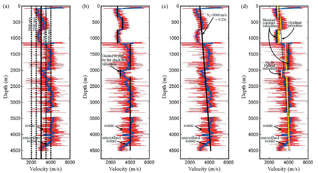
Figure 1 shows the sonic velocities and smoothed sonic velocities along with a series of velocity profiles. Four styles of velocity profile were constructed at the well: constant velocity (Figure 1a), constant velocities within distinct layers (Figure 1b), a velocity gradient (Figure 1c) and a hybrid model (Figure 1d). No single constant velocity fit the borehole data well, so we constructed a series of constant V₀ models: 2500, 3000, 3500, 4000, and 4500 m/s. The method of blocking the well into discrete layers and assigning constant velocity fits the borehole data well (Figure 1b). Where the blocked data appear to deviate significantly from the sonic curve, at approximately 2000 m depth, the velocity was picked in conjunction with the checkshot velocities. A third model considered that the velocities could be approximated by a linear increase in velocity with depth (Figure 1c).

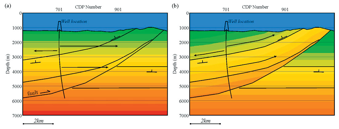
There is only a single borehole located on the seismic line therefore the additional velocities for the V₀ model were extrapolated from this borehole. Figure 2 shows the two methods of extrapolation that were used: V(z) and V(x,z). In the V(z) case, the velocities were extrapolated horizontally across the model, so that a V(z) medium was created. In the V(x,z) case, velocities were extrapolated along the interpreted bedding planes.

Consider the four velocity profiles obtained from the well. The constant velocity borehole profile (Figure 1a) results in a constant V₀ model regardless of the extrapolation method. When a velocity gradient approximates the velocities in the borehole (Figure 1c), the method of extrapolation becomes more important. The example shown in Figure 2 uses velocity gradients, and clearly shows that V₀ varies significantly between the models, especially in the dipping hanging wall strata. Specifically, a velocity inversion across the fault is seen in the V(x,z) example (Figure 2b), but not the V(z) example (Figure 2a). In the case of distinct layers containing constant velocity (Figure 1c), the only extrapolation method used was that along bedding planes.

In addition to the three models discussed above, a hybrid model was considered in which the velocities were partially a function of geology i.e. distinct layers, and partially a function of depth, i.e. velocity gradient. The velocities at the well for a hybrid model, that contained a 50% contribution to the velocity from a blocked model and a gradient model, is shown in Figure 1d. In effect, the resultant model is a blocked model that also contains a gradient within each layer. Figure 3 illustrates the well profile of Figure 1d projected into the model. The constant velocity layers are projects along bedding planes, and the velocity gradient is considered in this case to be a function of lithostatic load and therefore applied vertically to the model.

Anisotropy

We often make assumptions regarding anisotropy in the Vεδθ model, firstly, that the axis of symmetry, θ, is always perpendicular to the dip of the strata, and, secondly, that the velocity model comprises distinct layers of isotropic and anisotropic strata. In addition, the anisotropic layers are represented by a constant value. Further studies on the nature of anisotropy within stratigraphic layers are required but at this time seismic resolution does not allow for more detailed determination of the parameters.

There are many methods for estimating the anisotropy including laboratory studies, field measurements or data driven techniques (Newrick, 2004). A good initial estimate for anisotropy is ε = 0.12 and δ = 0.03 (Vestrum, 2005) but these values should be tested as the Vεδθ model converges to a solution and not simply taken as “the” values for interbedded sandstone and shale. Ideally, independent field measurements, such as refraction seismic, VSPs or borehole logs, should be used to obtain values of anisotropy, so that the magnitude and distribution within the model can be considered geologically reasonable.

The Vεδθ model is assessed and refined using imaging techniques, i.e. flattening image gathers to obtain a coherent stack, but iterations of the model should not deviate from the realm of geological reasonableness. In addition, the static solutions must be reconsidered as static solutions derived from time processing are no longer valid.

Weathering and model based moveout statics

A good approach is to incorporate the velocity model from weathering statics calculations directly into the prestack depth migration Vεδθ model. The weathering statics can then be removed from the traces, so that near-surface traveltimes are calculated within the migration. Weathering statics presently yield isotropic velocities therefore when anisotropy is included in the near surface the velocities should be reduced to a percentage, i.e. 95%, of the original velocities.

Traditionally, residual statics from time processing are applied to the input gathers, and the depth migration proceeds with these statics. But, depth migration uses a different velocity model to that of time processing, therefore, the statics are no longer coupled with the velocity model after depth migration. A solution to this is to remove the time processing residual statics so that depth processing statics can be calculated and applied. In time processing, the surface consistent residual statics are calculated after an NMO correction is applied to the gathers using the optimum velocity model. We apply a similar technique, except that the moveout correction to the gathers is based upon raytracing through the depth velocity model and hence the term model-based moveout (MMO) statics is used to refer to the technique. Effectively, a zero-offset migration is applied to the gathers. The MMO gathers are converted from depth to time, also using the depth interval velocity model, so that the surface consistent MMO statics can be calculated and then applied to the input shot gathers.

Ideally, a new set of MMO statics should be calculated with each new velocity model and migration run, but the additional processing time is prohibitive. Consequently, we only calculated and applied MMO statics in conjunction with a small subset of migrations. When model-based moveout statics (MMO) were included in the processing flow the CIGs contained reflectors that were more continuous, resulting in a more coherent stack.

Summary

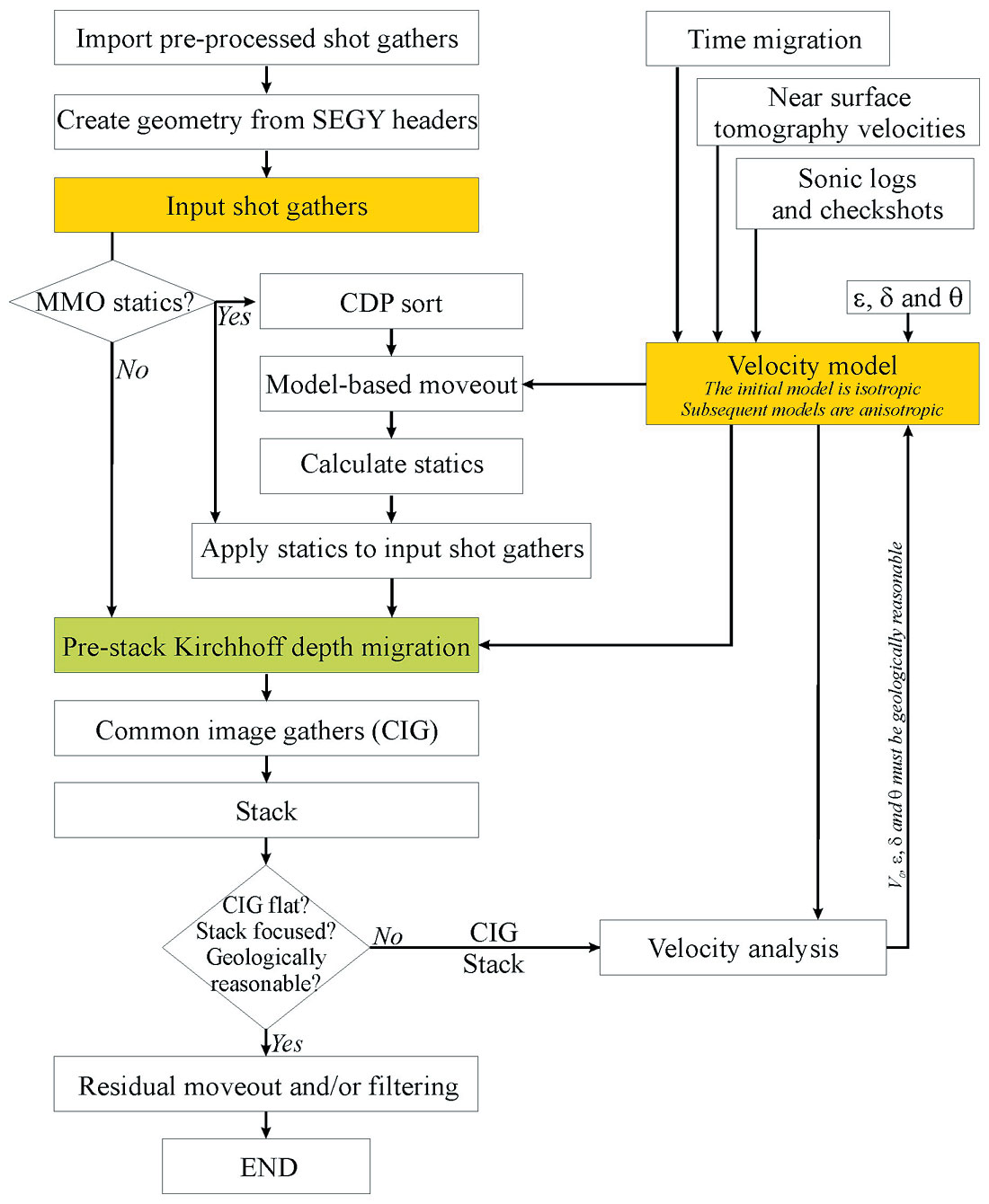
A prestack depth imaging procedure (Figure 4) that utilises a geologically reasonable Vεδθ model provides the interpreter with confidence that the migration parameters are appropriate and that the final image is robust. Interpreter input for depth imaging is critical and should be considered part of the interpretation process.

1. Gather all geological and geophysical information available.
2. Use all velocity input to construct a V₀ model.
3. Obtain independent measurements of the Thomsen parameters of anisotropy from laboratory or field measurements to build an initial ε and δ model. Use data driven techniques to guide Vεδθ model variations.
4. Construct a θ model based upon the style of transverse isotropy (i.e. vertical, transverse or horizontal).
5. Q.C. the migration output, i.e. common image gathers and stack, and vary the Vεδθ parameters to flatten common image gathers and focus the stack.
6. Iterate.
7. Confirm that the final Vεδθ model is geologically reasonable.
8. Calculate and apply depth static solution.

Acknowledgements

We would like to acknowledge the sponsors of the Fold-Fault Research Project (F2RP). Deborah Spratt and the staff and students of F2RP are thanked for their encouragement with this project.

We are especially grateful to EcoPetrol de Colombia and Occidental Petroleum Ltd. for providing the data. Time processing was undertaken at EPIC Geophysical under the guidance of Bill Leggett and depth processing was undertaken at Veritas GeoServices under the guidance of Rob Vestrum and Jon Gittins (now Thrust Belt Imaging) and the depth processing group. The use of model-based moveout (MMO) statics was first suggested to us by Al Petrella at Veritas GeoServices.

We thank Nexen Inc. for encouraging the presentation of this material at the CSPG structure division and CSEG technical luncheons.