Over time, Geophysics, like most disciplines and industries have developed a veritable arsenal of powerful software tools to defeat complex modeling and analytical challenges. Whether the task is contouring, groundwater modeling, or GIS, highly capable software exists to help today’s problems. But what about the problems of tomorrow?
This article presents a case for “de-specialization” – that is, applying software tools meant for a more general audience in a highly specialized context. In other scientific and engineering arenas like the auto and aerospace industries, people are starting to experience the limits of the conventional software tool set. CAD, dynamic simulation, and automatic control, are just a few of the areas that are being stretched by emerging new product initiatives such as green vehicles or “active”-whatever. Many in these industries are currently opting to go the de-specialized route for software – using tools that have the power to ultimately solve the analytical problem but have a chameleon quality that allows it to be easily reconfigured for vastly different applications.
Maple from Maplesoft is an example of a general tool making waves in the auto and aerospace industries. Originally conceived in the 80’s as a detailed programming language for high-end mathematics, it has recently evolved to become a flexible modeling platform for a wide variety of math-based models – the primary forms in auto and aerospace, consequently, were very adaptable to this platform. The advantage of this approach is profound.
- Many emerging analytical techniques are inherently and deeply mathematical and Maple offers streamlined tools to implement these.
- There are a wide range of visualization tools that can quickly be adapted to a vast range of modeling activities.
- Convenient data interchange and connectivity tools allow it to merge with many existing tools to ensure a smooth growth path.
- Documentation and reporting tools facilitate easy documentation of densely technical information
- Cost is often significantly lower than highly specialized tools.
Case study: Modeling the Magnetosphere with Maple
The following example shows how Maple was readily adapted for an application in geophysics. It is a clear example of the flexibility of the system for modeling applications that the system was not initially designed for.
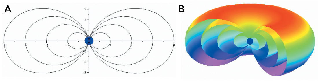
The magnetosphere is the area of space around the Earth that is controlled by the Earth’s magnetic field. The earth’s magnetic field protects our atmosphere from the charged particles ejected from the sun. The force of this solar wind deforms, or squashes, the earth’s magnetic field as the particles are slowed down and deflected by the earth’s magnetosphere. Without this protection, the earth’s atmosphere would be continuously eroded into space. Since the earth is, in essence, immersed in the sun’s atmosphere, as it moves through the solar wind, the magnetosphere is distorted. Charged particles interacting with the earth’s magnetic field lines can give rise to vivid auroral displays, radio and television interferences, and erratic compass behavior. More severe conditions can even cause power blackouts.
1b. 3D Approximation of the Magnetosphere without Solar Wind Effect.
How was it done?
Maple was used to mathematically describe the Earth’s magnetosphere. It involved an analytical model of the interaction between the solar wind and the earth’s magnetic field. This allowed for plotting and visualization of the relevant phenomenon directly from the model. Once the 2D representation was found, a 3D approximation was also solved for.
The magnetic field around the earth is broken down into two main components, the earth’s innate dipole magnetic field, and field created by its interaction with the charged particles from the solar wind. The magnetosphere itself is the distribution around the earth of this magnetic field composed of these two sources.
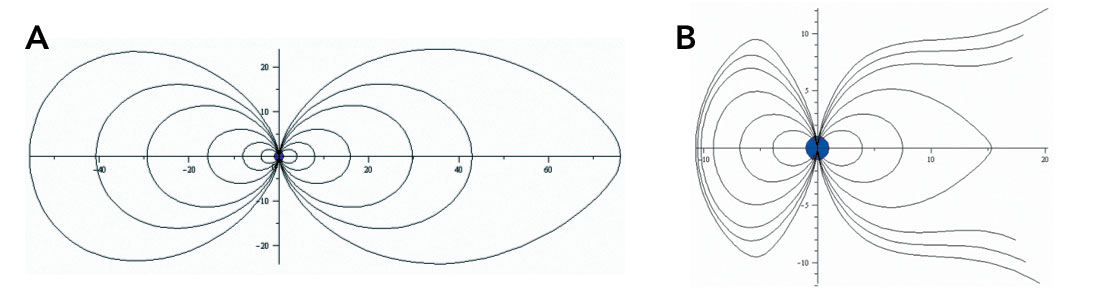
Figure 2b. Magnetic Field Lines for a Strong Solar Wind Intensity
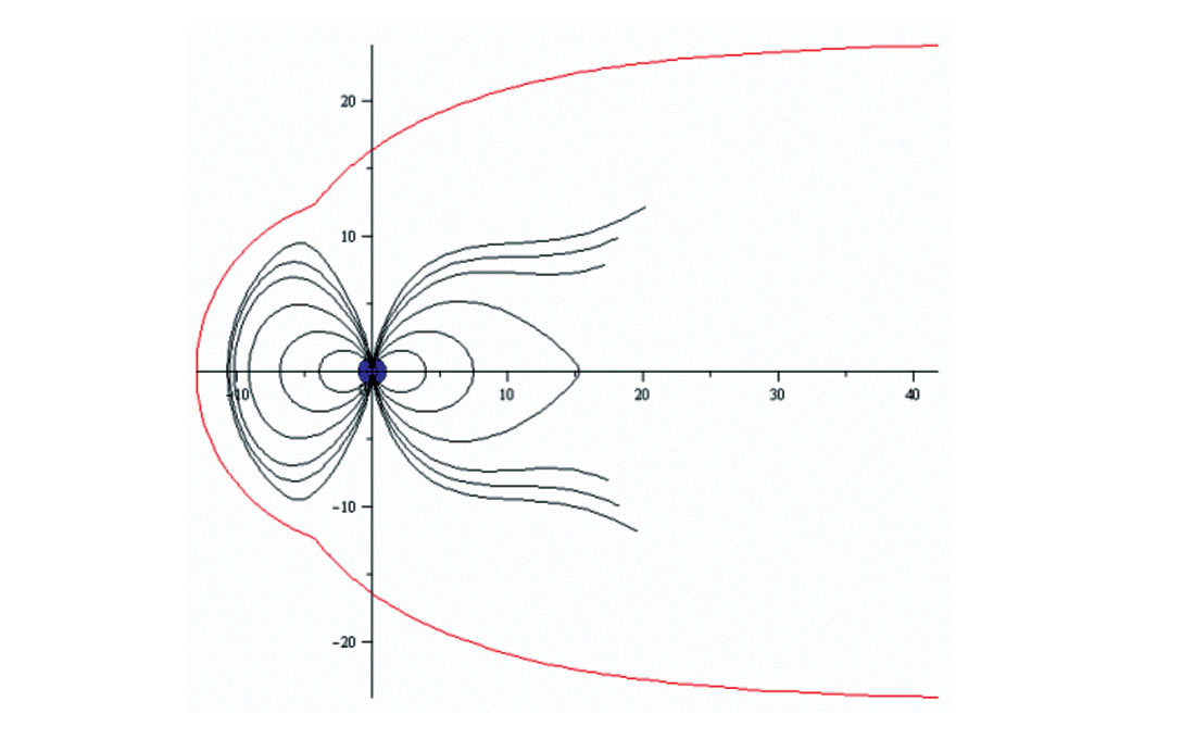
The magnetopause is the delimited border of the magnetosphere, which exists because of the solar wind. Any significant magnetic field is only observable within the magnetopause. The mathematic model in Maple represented analytically the distribution of the magnetic field within the magnetopause, as well as the magnetopause itself.
The Maple model considered the earth as a point and the magnetic field lines to start at the origin. To visualize, the earth was represented as a blue disk at the origin:
Two Maple procedures were written for the analysis: PlotMagneticFieldLine and PlotMagneticFieldSurface. Working with these two procedures, it was possible to create a sequence of plots representing magnetic field lines and their corresponding magnetic surfaces, and see the changes in the magnetosphere as the intensity of the solar wind was increased. As the intensity of the solar wind increases, the magnetic lines in the side of the magnetosphere closest to the sun become more compressed, and the magnetic lines in the dark side become elongated, even breaking (representing the magnetotail which closes at infinity).
Using the simplified model, it was also possible to create a formulation of the magnetopause, the delimiting border around the magnetosphere. A plot of the magnetopause may be seen in Figure 3.
Making it simpler and faster
The first objective of creating a simplified analytical model was to see how one could visualize the relevant phenomena directly from an analytical model, allowing it to be compared to empirical data. The second was to produce a related document with active mathematical expressions in the form of a Maple document, and discuss the techniques of how the problem can be modeled in such a framework.
A great advantage was that all the activity took place in the same computational environment, without having to master numerical techniques or other programming computer languages. This approach can provide adequate understanding and prediction capabilities without resorting to classical brute force finite element and finite difference simulation models. Taking advantage of Maple’s power saved enormous amount of time and also made the complex process much easier. Maple documents capture the analytical modeling as well as numerical experiments, supported by an efficient computational engine.
The ultimate irony
As recent as 30 years ago, scientists were forced to do every computing task from scratch. We had to program our own equation solvers, our own user interface, data collection, etc. Then came the era of the specialized tools that ruled the computing landscape for the next decades. They had the power and stature of almost Jurassic proportions. Eventually though, their complexity and cost are starting to trigger discussions and even challenges. Through all of this, the nimble, even humble, general math tools are once again making a difference. Yes, you do have to build some things yourself again but one major difference between today’s general purpose tools like Maple and the “do it yourself” FORTRAN era is that the new tools still embody the focus on ease-of-use and accessibility that is characteristic of all good modern software applications. You get gain and relatively little pain.


Join the Conversation
Interested in starting, or contributing to a conversation about an article or issue of the RECORDER? Join our CSEG LinkedIn Group.
Share This Article