Fast Search Algorithms for Automatic Localization of Microseismic Events

Abstract

Automatic localization of microseismic events has become an important tool in characterizing formations which generate large numbers of microseisms during hydraulic fracturing, e.g. Horn River shales. Especially for large complex threedimensional velocity models, the automatic processing requires the use of specialized optimization algorithms to locate the events within an acceptable timeframe, i.e. usually in a few seconds. Regular grid searches are very thorough and always find the absolute best fitting event location. But these algorithms are very slow and only practical for small, i.e. two-dimensional, grids. The number of grid points in three-dimensional models slows down the standard algorithms too much for real-time localization or optimization. Meta-heuristic search algorithms like Artificial Bee Colony and Differential Evolution provide a best-fit solution with much fewer calculation steps and are well suited for automatic event localization and velocity model optimization. Examples from different datasets compare the automatic realtime results using the different search and optimization algorithms and point out some pitfalls in their application and provide some guidance in choosing the best search strategies.

Introduction

Automatic localization of events is a standard technique in global seismology to locate earthquakes recorded on a network of distributed stations (e.g. Bai, Kennett, 2000; Earle, Shearer, 1994). Usually these methods require the prior identification of P-wave or S-wave arrivals. Methods have been developed to identify different phases at individual stations (e.g Sleeman, van Eck, 1999; Ton, Kennett, 1996) which also can be applied to microseismic recordings. Some of these methods can be adapted to the special acquisition geometry of microseismic downhole sensor arrays (e.g. Xuan, Sava, 2010). But any method requiring the prior identification of Pand S-wave phases on a single 3-component geophone does not make use of the long strings of geophones typically applied in downhole microseismic mapping. An alternative approach especially suited for automatic processing is the use of migration or refraction stacks which is now routinely applied to locate microseismic data as this technique does not require prior knowledge of the phase arrivals (e.g. Drew et al., 2005). The arrivals of P- and S-waves are provided as an output once the most likely event location is determined.

Objective functions for event localization

The objective function translates the given problem, here the localization of a microseismic event, into numbers in the solution space ( here the grid points of all possible event locations) so that the absolute minimum (or maximum) describes the most probable solution. The objective function for locating a microseismic event can be defined in many different ways. When processing a microseismic event manually, often the first arriving P- and S-waves are identified in the recordings and their traveltimes are marked. These picked traveltimes are then compared to the theoretical arrival times from all the potential event locations, typically defined as a three-dimensional grid. The grid point where the difference between the picked traveltimes and theoretical traveltimes is the smallest is considered the most likely event location. For automatic processing, a different approach is often employed.

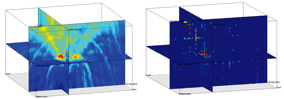
For automatic processing, the theoretical arrival times for each grid point to each sensor are used as templates. These templates slide over the waveform record of a potential event and the signal along the templates for each grid point is added up. The maximum stacking result is then assigned to the grid point providing a measure of the probability that an event from this record is located in that point. Repeating this procedure for all grid points provides a (volume) map where the grid point with the maximum stacking result is the most probable event location. Different authors use different signals in the stacking process. Garthi et al. (2010) use the Hilbert transform of the 3-component waveform, Drew et al. (2005) use a different combination of the 3- component amplitude traces. In the examples below the energy ratio with a series of additional filtering and weighted by the hodogram, i.e. particle motion observed at the sensor, is used. Whatever objective function is defined, the result will be a value distribution as shown in Figure 1 where the point with the maximum value identifies the most likely event location. Depending on the definition of the objective function the pointof- interest could be identified by either the global maximum or global minimum. In the following examples the objective function used requires the identification of the global maximum. But the subsequent search algorithms work equally well for objective functions where the global minimum needs to be identified.

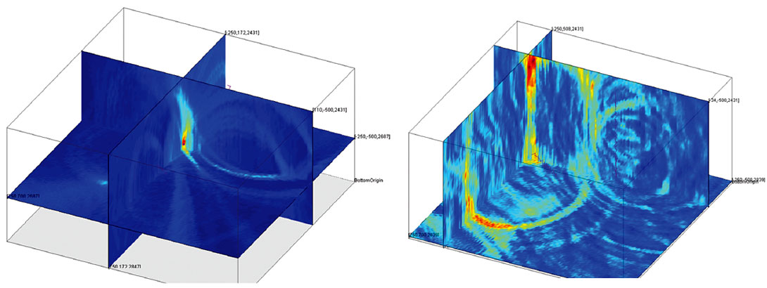
Figure 1 shows two examples of objective functions from real events. The objective function on the left is from an event with a large signal-to-noise ratio and only a single P-S wave pair in the recording. Consequently, the objective function shows only a single well-defined maximum. On the right side the objective function from a more typical event with P- and S-waves showing a much lower signal-to-noise ratio has multiple local maxima that are almost as strong as the overall global maximum.

Another example (Figure 2) shows the waveforms and the associated objective function for a 12 level sensor array. This objective function shows multiple maxima of almost equal height. This is a consequence of the waveforms showing not just a clear P- and S-wave arrival pair but a coda of multiple secondary arrivals.

Search algorithms

In order to locate an event, the grid point with the global maximum of the objective function needs to be identified. This is a typical optimization problem and many different algorithms exist to solve such a problem quickly. In the following, different algorithms are evaluated and although this list is by no means complete or even extensive, it shows that some algorithms perform better than others for the given type of problem. Other search algorithms include Particle Swarm Optimization (PSO), Ant Colony Optimization, Firefly Algorithm, Monkey Search and Cuckoo Search.

Linear grid search

The most straight forward way to find the global maximum of a distribution is to evaluate every single grid point, i.e. linear grid search. This method has the advantage that it always finds the global maximum, i.e. the most likely event location. For small grids, usually two-dimensional, this method is very useful but the time to find the solution is direct proportional to the number of grid points which makes it prohibitively slow for large three-dimensional grid spaces typical for microseismic event localization.

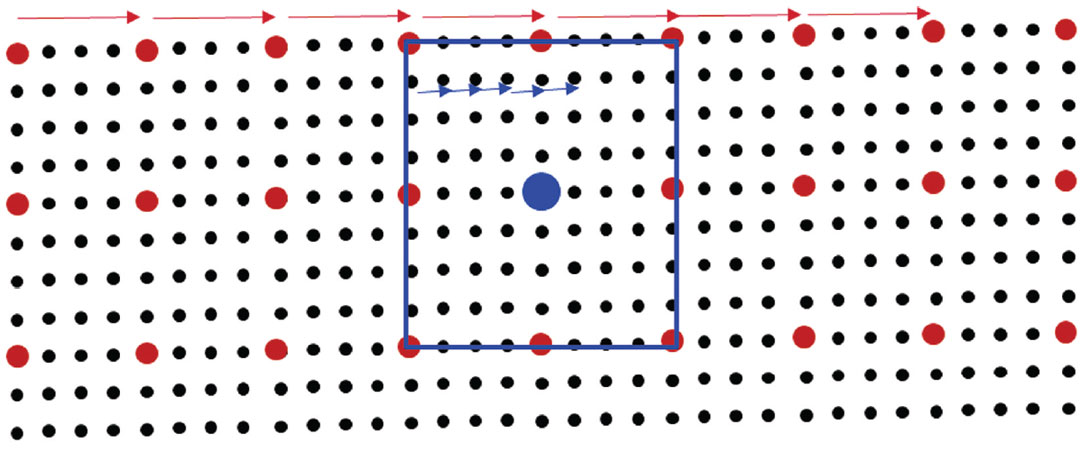
Figure 3 shows a schematic visualization of the linear grid search and a modified version. To speed up the search it is possible to initially evaluate only every nth grid point and then refine the search when a potential global maximum is encountered. This approach requires that the global maximum of the objective function is smooth between the skipped grid points. Although this variation of the linear grid search speeds up the search process and most often finds the correct global maximum, provided that the initial search is not too coarse, it also runs into time issues for realtime processing of a steady stream of microseismic data.

Gradient based methods

The conjugate gradient method is often used as an iterative algorithm to find the numerical solution to a system of linear equations. But the method can also be used to solve unconstrained optimization problems such as finding the maximum of a distribution. The method is described in detail in many computer mathematics textbooks (e.g. Meurant, 2006). An intuitive description is provided by Shewchuck (1994). Unfortunately, the conjugate gradient method and similar methods cannot be applied in this particular case as it requires an objective function that is differentiable everywhere and has only one (local and global) maximum. As can be readily seen from the examples provided (Figure 1 and Figure 2) neither assumption is valid for the objective function in these cases.

Meta-heuristic Algorithms and the ‘free lunch’ theorem

Since gradient based methods do not work in this case, other methods are required to speed up the grid search. According to Luke (2009) meta-heuristic search algorithms are “a common but unfortunate name for any stochastic optimization algorithm intended to be the last resort before giving up and using random or brute-force search. Such algorithms are used for problems where you don't know how to find a good solution, but if shown a candidate solution, you can give it a grade”. Meta-heuristic methods do not search the grid space in a linear fashion but only search a very small portion of it. They usually start out by evaluating the objective function on a limited number of grid points. Based on these results, new grid points are selected for evaluation. This process is repeated until a convergence criterion is reached. The different methods differ in the way these three basic steps are implemented. All of these methods are not guaranteed to find the global maximum, but for objective functions that do not vary too quickly, they often converge to the correct solution.

The ‘No free lunch theorem’ according to (Wolpert, Macready, 1997) states that “All algorithms that search for an extremum of a cost function perform exactly the same when averaged over all possible cost functions”. If this theorem would apply to the given problem it would mean that over time there will be an equal amount of events that successfully and unsuccessfully processed with any of the implemented meta-heuristic methods. Fortunately this is not the case for the given objective functions as their variation between grid points is limited largely by the limited frequency content of the waveforms. In such a case the method that is most optimized to the objective function will provide the most reliable results. In the following, three search algorithms are tested.

Simulated Annealing (SA)

As with all meta-heuristic search algorithms, Simulated Annealing can be implemented in different variations depending on the chosen parameters and procedures. But in general, simulated annealing (SA) starts out with an arbitrary distribution of grid points scattered over a certain area (Figure 4 (left)). The object function at these grid points is evaluated and a grid point, usually the point with the best fit, is chosen as the center of the new population of grid points (Figure 4 (right)). This new population covers a smaller area. These steps are repeated until either the extension of the population is smaller than a certain threshold or the maximum number of iteration steps is reached.

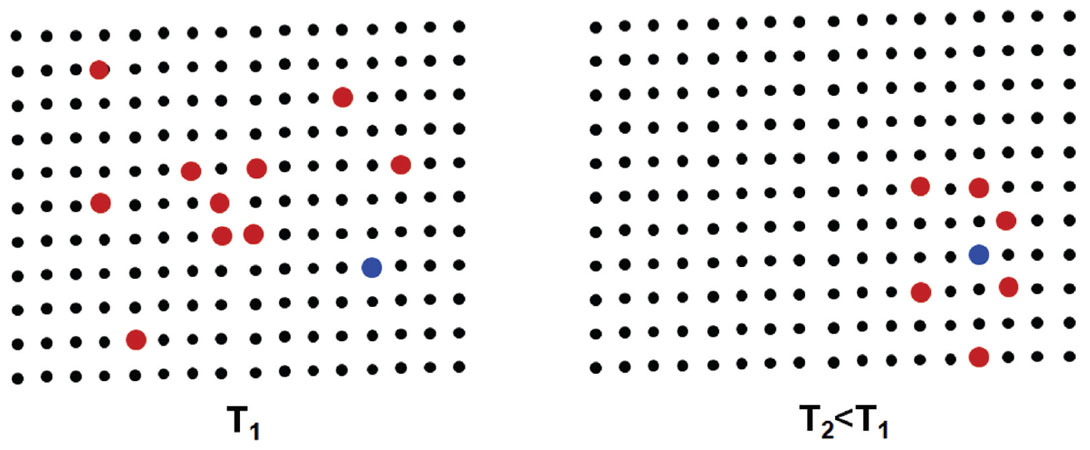
Figure 5 shows the results of applying the simulated annealing algorithm to a real data objective function. On the left the full three-dimensional objective function is displayed. On the right side the same objective function is used but only a very limited number of grid points are evaluated before the search algorithm converges to the global maximum. Since only a very small percentage of the grid points need to be evaluated, the result is obtained much faster than the linear grid search.

Artificial Bee Colony (ABC)

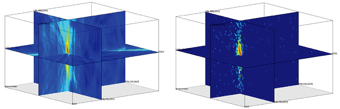
The Artificial Bee Colony (ABC) algorithm is a swarm based meta-heuristic algorithm that was introduced by Karaboga (Karaboga, Basturk, 2007, 2008; Karaboga, 2010) for optimizing numerical problems. It was inspired by the intelligent foraging behavior of honey bees looking for the best food source, i.e. optimum solution. The algorithm employs three different types of bees. Employed bees search the vicinity of existing food sources, i.e. good solutions. They also report back to the other bees about the quality of the food source and try to recruit other bees to their area. The onlooker bees back in the hive prioritize the information of all the employed bees and depending on this information can become employed bees recruited to a specific food source. Once a food source is exhausted the employed bees become either onlooker bees back in the hive or scout bees that randomly choose a new food source. The algorithm declares the current best food source the optimum solution once most bees are recruited to it. The specific behavior of the algorithm can be controlled through the initial number of bees and the probabilities with which they switch between different roles. Meta-heuristic algorithms try to balance between the exploration of the solution space and the exploitation of the vicinity of existing good solutions. Figure 6 shows an example of an objective function from another event. The complete function, which is the result of a time consuming linear grid search, is shown on the left side where the results of the ABC search are on the right. Similar to the results of the simulated annealing algorithm (Figure 5) the ABC algorithm also converged fast to a solution but was on average more reliable in finding the correct solution than the SA algorithm.

Differential Evolution (DE)

Differential Evolution (DE) is an algorithm that recently has received some attention for its use in automatic event location (Gharti et al. 2010, Zimmer, Jin, 2011). Figure 7 schematically shows how the algorithm works. Similar to the ABC and SA algorithms the differential evolution starts with an initial population of grid points (x). For a random point in the population three other points are chosen and a new point (U) is constructed according to the equation shown in Figure 7 which is termed the ‘search strategy’. Other equations determining different search strategy can be used and their success depends on the shape of the objective function. In addition, by varying the different parameters of the implemented search strategy the algorithm can be optimized for very different datasets. Although the algorithm is very flexible and can be adapted to different datasets, tests have shown that a stable performance of the algorithm can be achieved with a standard set of parameters. If the new point U indicates a better fit, i.e. high value of the objective function, than the original point Xj, it replaces the original point. This procedure is repeated for every point in the original population. One of these cycles through all the population points is termed a ‘generation’. This iterative process is repeated until a set number of generations is reached or the scatter of the population points is below a set threshold. An extensive discussion of the Differential Evolution algorithm including different search strategies can be found in Feoktistov (2006).

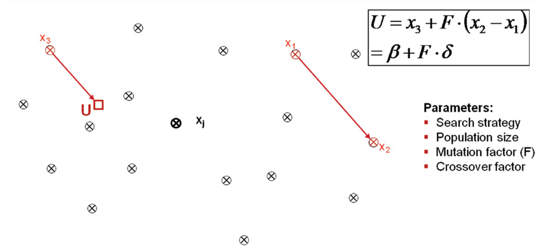
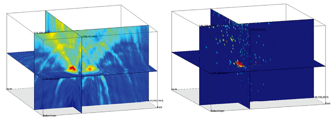
Figure 8 shows the complete objective function on the right and the result of the differential evolution search on the left. The DE algorithm quickly converged to the correct solution and proved very reliable on different type of objective functions.

Summary and Conclusions

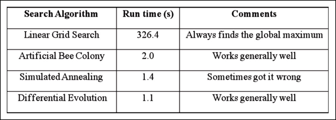
Table 1 summarizes the results for the different search algorithms tested. As expected the linear grid search was the most reliable algorithm but its required run time of more than 5 minutes for a single event on the test grid makes it prohibitively slow for realtime processing. The meta-heuristic search algorithms perform faster by more than two orders of magnitude. Since these methods do not search the full grid space they are not guaranteed to find the global maximum of the objective function but most of the algorithms worked very well. The Differential Evolution (DE) and Artificial Bee Colony (ABC) algorithms usually converged quickly to the correct solution with the DE algorithm performing quicker than ABC. The Simulated Annealing (SA) algorithm was almost as fast as the DE algorithm but did not perform as reliably. The performance of all metaheuristic algorithms can be significantly influenced by the choice of their parameters. Depending on the dataset, even Simulated Annealing, which provided the worst results, can provide decent results by adjusting its parameters to the individual dataset. In that respect the results in Table 1 should not be over-interpreted. However, from our experience with real data thus far, the Differential Evolution algorithm provides good results with minimal adjustment to the individual datasets. So far, the DE algorithm has been successfully applied in the automatic processing of hundreds of individual stage treatments and has proved its practical suitability for automatic real-time localization of microseismic events.

Although the linear grid search is the slowest of all the tested algorithms its ability to always find the global maximum of the objective function makes it still an interesting method for small two-dimensional grids or where speed is not a crucial factor. For large three-dimensional grids meta-heuristic algorithms have clear advantages over linear grid searches. For formations that produce large numbers of microseismic events, the added performance in locating the events using meta-heuristic search algorithms might not be sufficient to process all the data in real-time. In such cases criterions such as average signal-tonoise, recording time or other project specific criteria can be used prioritize the events. Although not guaranteed to find the global maximum, their fast performance and typical good results makes meta-heuristic search algorithms an excellent choice for automatic realtime processing of microseismic events.

Acknowledgements

We thank Prof. Karaboga for generously providing us with the latest version of his Artificial Bee Colony (ABC) code. We also thank Dr. Kenneth Price and Dr. Rainer Storn for sharing the latest version of their Differential Evolution (DE) algorithm.