Estimating Intrinsic Layer Anisotropy η_layer From Surface Seismic

Abstract

The anisotropic parameters (V_nmo , η_effective) are now routinely and robustly estimated from anisotropic prestack time migration velocity analysis. The availability of these parameters opens the possibility for determination of parameters potentially valuable for interpretation, such as layered intrinsic anisotropic layer η_layer.

In this work, we demonstrate the value and robustness of current anisotropic prestack time migration velocity analysis with two production data examples. The further steps to construct layered intrinsic η_layer from (V_nmo , η_effective) are then presented. Finally, for the two real data examples the dense layer intrinsic ηlayer is calculated. Inspection of this intrinsic property reveals it to be reasonably layer and structure consistent, with interesting potential to be an anisotropy-sensitive attribute for interpreters.

Introduction

The value of high quality, high density imaging velocity has been documented for nearly all aspects of interpretation and analysis, including basic structural and stratigraphic interpretation, overpressure analysis, 4D work, and others. To reliably and repeatably satisfy velocity determination needs, a data driven automatic approach was developed (Stinson et al. (2004), Stinson et al. (2005)) based on quantifying the quality of the migration velocity using objective measures derived from both the image gathers and the image cube. The automatic iterative optimization of these objective measures to determine migration velocity was shown to be robust, repeatable, and convergent, and the combined benefits of the objective data-driven approach, the optimization methodology, and the high density (in space and time) resulted in improved time migration images.

In later extensions, determination of the higher order moveout for curved ray time migration was included in the same methodology, with simultaneous estimation of the migration velocity and the higher order terms due to vertical velocity heterogeneity and intrinsic VTI anisotropy. Anisotropic curved ray time migration imaging and velocity analysis is now common in production work, with dense estimation of the time migration parameters V_nmo and η_effective.

Up to this point, our interest in the migration parameter fields V_nmo and η_effective focused mainly on their efficacy in imaging the data. Now, with garnered confidence from experience, we turn our attention to the determination and possible interpretative value of underlying physical values, such as the interval or layer values of η_layer due only to the intrinsic anisotropy.

We begin with two production data examples: the first a 2D section and the second a 3D cube. In both, the improvement in the migrated image is noted when effective anisotropy is estimated and included in the migration. However, our interest will be centered on V_nmo and η_effective sections that were necessary to produce the improved images.

Curved Ray Anisotropic Migration Velocity Estimation: Example #1

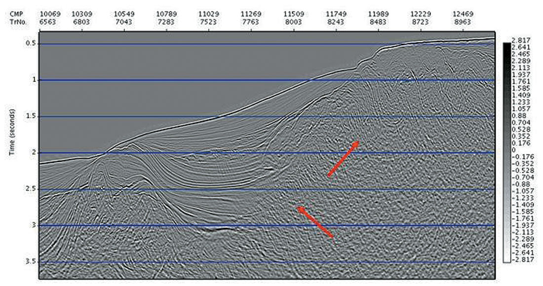
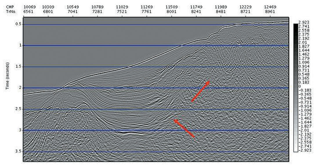
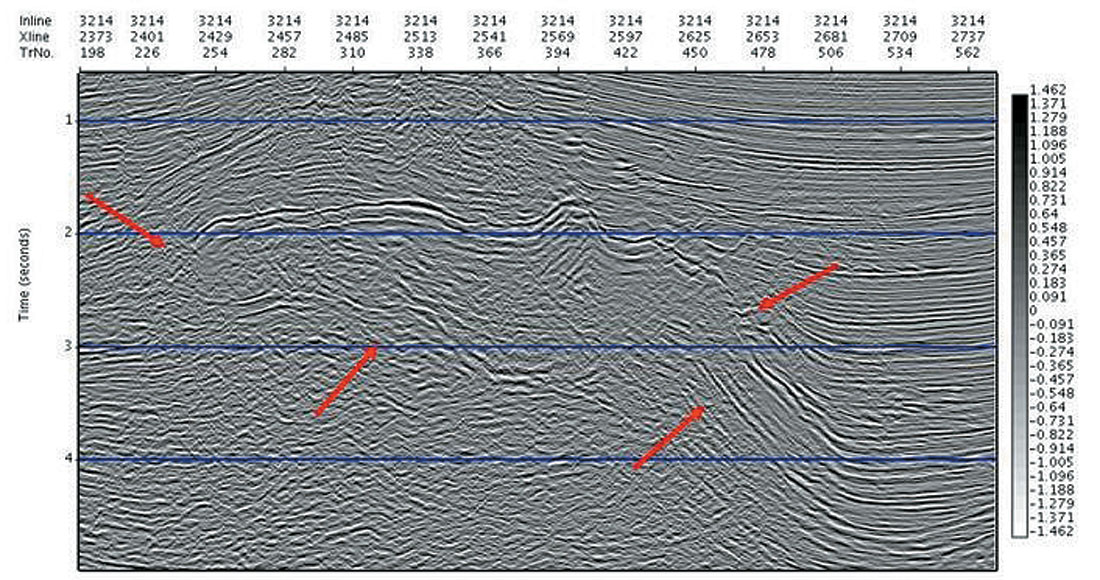
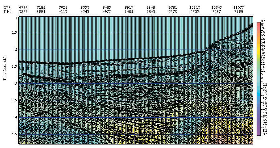
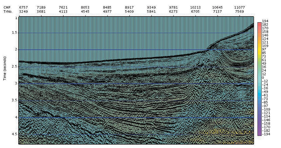
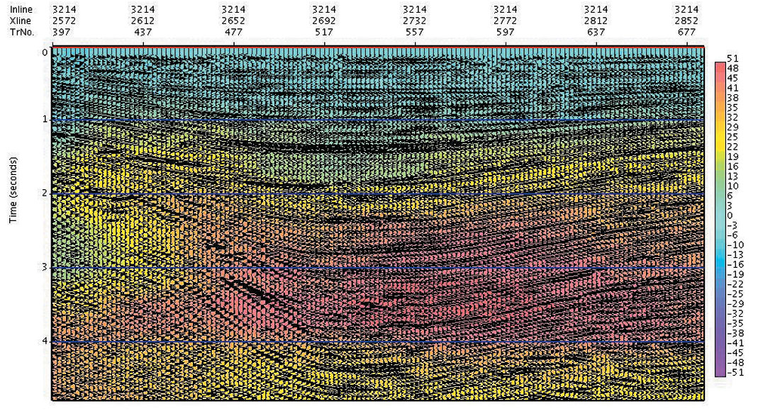
In the first example (a 2D regional line), we see in Fig. 1a the straight ray time migration, in which the optimized, dense hyperbolic migration velocity has been estimated.

In comparison, Fig. 1b shows the anisotropic curved ray time migration result, where the migration velocity V_nmo and effective anisotropy η_effective have been simultaneously determined. The red arrows mark the areas of obvious improvement (where steep events abut flatter events), but in fact we expect the position of all dipping events to be improved, and the imaging to be universally better focused.

To quantify our anisotropic moveout, we have used the non-hyperbolic moveout approximation for weak VTI anisotropy and vertical velocity heterogeneity introduced by Tsvankin and Thomsen (1995) and included in Alkalifah (1997):

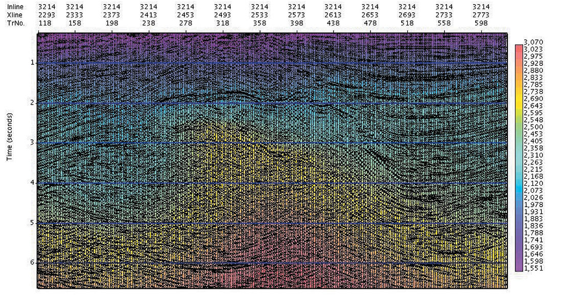
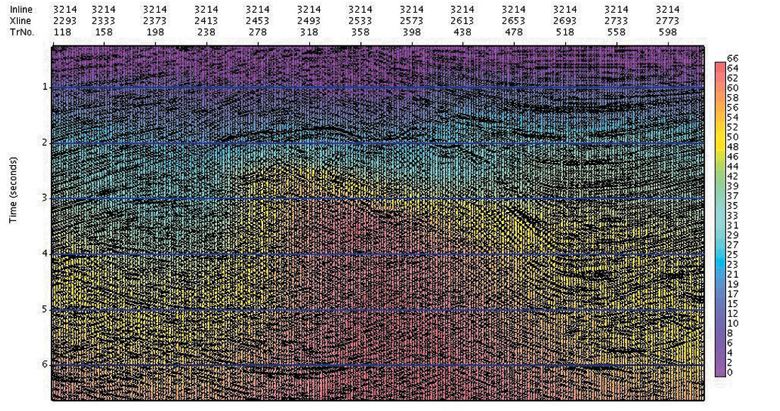
In the formulation of Equation 1, the higher order parameter η_effective describes the curved ray moveout component due to total apparent anisotropy from both vertical velocity heterogeneity as well as actual intrinsic VTI anisotropy. Shown in Fig. 1c and 1d are the estimated V_nmo and Total Effective η fields, respectively, for the first data example. Note the stability of the Total Effective η field, and its tracking of events and structure as demanded by the data (note that all values of η_effective in the colour sidebars of the plots have been multiplied by 1000 for ease of viewing).

Curved Ray Anisotropic Migration Velocity Estimation: Example #2

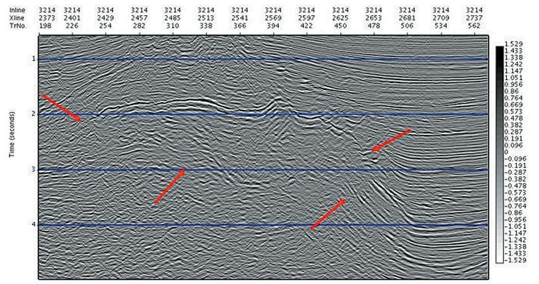
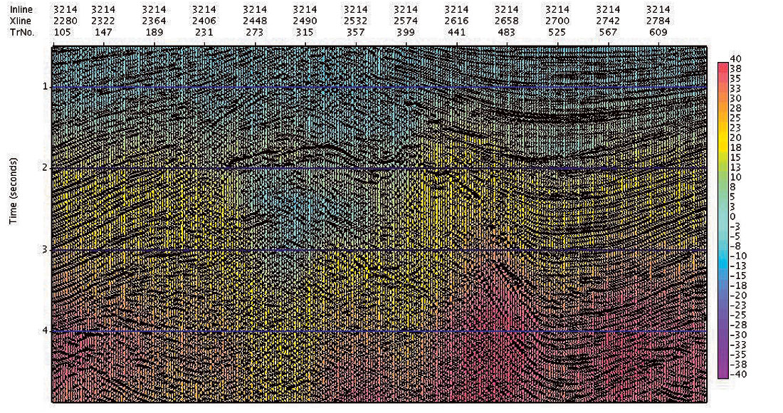
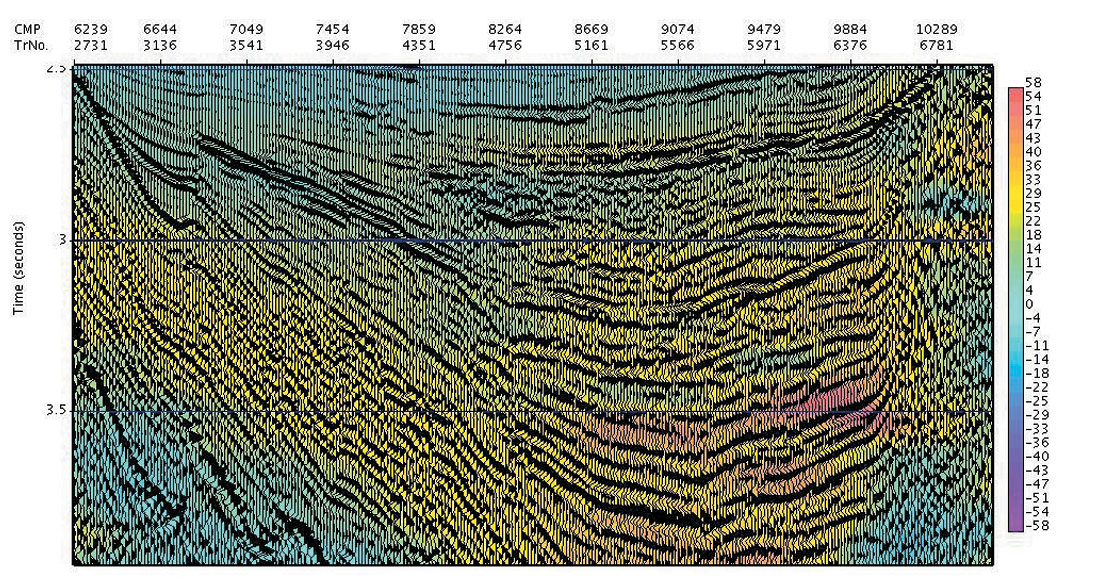
In the second example (from a marine 3D), we see in Fig. 2a a selected line from the straight ray prestack time migration cube (using the automatically determined dense migration velocity), and in Fig. 2b the curved ray time migration result, in which we have determined simultaneously the cubes of migration velocity V_nmo, and Total Effective η. The red arrows mark areas of improved imaging and positioning: the nose of the salt on the left hand side is both more clearly imaged and also the sediments now terminate naturally against it. The bottom of the salt, and on the right hand side the steep flank are also clearer.

Shown in Fig. 2c and 2d are the estimated V_nmo and Total Effective η fields, respectively, for this selected line from the 3D cube. Again, we note the stability of the Total Effective η_effective field, and its tracking of events and structure as demanded by the data.

Solving for Underlying Intrinsic Anisotropic Parameters:

Step 1 – Determination of Effective Intrinsic Anisotropy

The quality of the estimated dense anisotropic migration fields is evidenced by the improved images, and by the stability and structural consistency of V_nmo and Total Effective η. This compels and allows us to attempt further extraction of the underlying intrinsic layer anisotropy parameters. As a first step in this process, we recognize that our measured Total Effective η has a component of apparent anisotropy due to vertical velocity heterogeneity, and a component due to actual intrinsic anisotropy (presumed to be VTI), as per Tsvankin and Thomsen (1995) and Alkalifah (1997):

We may solve for the component of Effective anisotropy due only to the vertical velocity heterogeneity using:

This allows us to estimate the component of the Total Effective anisotropy due only to actual, intrinsic anisotropy using:

It is noted that η_intrinsic is still a weighted time average of the anisotropy to the given time ‘t₀’, and so includes the averaging effects of travel through all anisotropic layers above (much like the RMS velocity at a given time is the RMS average of the interval velocities of all layers above).

In Figure 3a we show a zoom of part of the 2D migrated image seen in Fig. 1b, with an overlay of the calculated intrinsic anisotropy, η_intrinsic. We again see the robustness of the result, with η_intrinsic tracking structure and events.

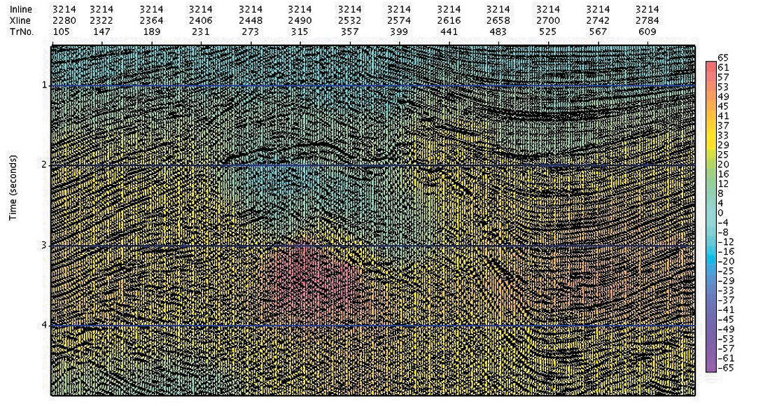
Similarly, we have for the previous 3D data example a zoom of the selected inline from the curved ray migration cube (Fig. 2b) with η_intrinsic overlain in colour, in Fig. 3b. We again note the general tracking of structure and layers.

Step 2 – Determination of Layer Intrinsic Anisotropy:

As per the development in Alkalifah (1997), the intrinsic anisotropy η_intrinsic we have calculated and shown in Step 1 above, is a weighted integral average of the intrinsic layer anisotropy:

where ν(τ) is interval velocity as a function of time.

This integral relation may be inverted to solve for the intrinsic layer anisotropy, η_layer(t₀), as we are in possession of the kernel function components (V_nmo(t₀), ν(t₀), and t₀). We recognize at the outset that as our input data to the inversion is a weighted integral average of the desired layer property, it will be a smoothed version of the layer function. In counterpoint, this tells us that η_layer(t₀) will likely be much more structured in time. (For a discussion of this and inherent non-uniqueness in the very similar problem of RMS velocity inversion, see Oldenburg et al., 1984).

Using the previously determined V_nmo(t₀), interval velocity ν(t₀), and intrinsic anisotropy η_intrinsic (t₀) for the previous 2D data example, we invert for the intrinsic layer anisotropy η_layer(t₀). Shown in Figure 4a is a zoomed portion of the 2D migrated line, now with η_layer overlain in colour (it is noted again that values in the colour side bar have been multiplied by 1000 for ease of viewing).

From the larger scale view of the 2D data set in Fig. 4a, we see that our constructed η_layer appears to be stable and generally structurally consistent. To get a feel for potential interpretational value of this new anisotropy attribute, we zoom in on the basin, in Fig. 4b below.

The observed layer consistency of η_layer intriguingly offers that the local lateral variations in this local measure of anisotropy may be interpretationally significant and useful (perhaps in terms of identifying fracture orientation). In Figure 4c below, we inspect another small basin, on the far right of this regional 2D line (not visible in Fig. 4a). Again, the general layer and structural consistency of this estimate of layer intrinsic anisotropy makes this measure very interesting.

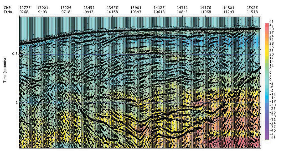
For completeness of our two data examples, we follow the same construction and inversion steps for the selected line from our 3D data example. Shown in Fig. 5a is the determined η_layer for this line (again overlain in colour on the anisotropic curved ray migration result). As with the 2D result, we note the apparent structural integrity of the calculated local anisotropy attribute, η_layer. A closer zoom of the right hand basin (Figure 5b) further indicates the layer and structure consistency of the result.

Summary

Anisotropic time migration velocity analysis is routinely utilized to robustly determine V_nmo and Total Effective η for anisotropic curved ray prestack time migration. The quality and density of these determined parameters (as seen on a 2D and 3D production data set) leads us to pursue the further extraction of layer intrinsic anisotropy. A methodology for separation of the Total Effective η into its components (one due to vertical velocity heterogeneity and the other from intrinsic material anisotropy) is presented, with the underlying assumptions that lateral velocity variations are not severe (required for time migration as well) and that the intrinsic anisotropy is VTI only. The intrinsic material anisotropy measure (η_intrinsic) derived for the two real data sets is robust and is seen to generally follow structural and layer trends.

The intrinsic anisotropy measure, η_intrinsic(t₀) derived above, is a weighted integral average from surface to the image ray time ‘t₀’, and so will not easily reveal local properties at ‘t₀’. A more desirable interpretative function is the interval or layer values of the intrinsic η: η_layer(t₀), which will more readily reveal vertical and lateral changes in the intrinsic anisotropy.

The integral relation between the time averaged η_intrinsic(t₀), and the interval η_layer(t₀) is solved for the 2D and 3D production data examples, with the resulting η_layer fields displaying structural and layer consistency. These observed features suggest the measure is robust and meaningful, giving us potentially an interpretable local intrinsic anisotropy measure at the seismic scale.

Acknowledgements

We thank Geophysical Service Incorporated for access to the 2D data set and for allowing us to show it. We similarly thank Petroleum Geo-Services for allowing us to use and show results for the 3D data set.