Effect of Well Control on Constrained Sparse Spike Seismic Inversion

Abstract

Modern seismic inversion methods transform seismic reflection data to pseudo acoustic impedance logs. Implicit in this approach is an integration of low frequency model information with higher frequencies from the seismic. This is necessary since the low frequencies present in logs and therefore required by the inversion, are absent in the seismic data. We obtain the low frequency impedances from a 3D solid model defined by interpreted horizons and impedance logs. It is important to understand the effects of this a priori log information on the final inversion. We must guard against using the logs to provide the answer. Our goal is to place the transformed high frequency seismic information in a reasonable geologic setting defined by the low frequency model.

We investigate these ideas using a western Canadian example, a small 8600 bin 3D survey over a Devonian reef. Within it are located 19 wells, each with a set of sonic and density logs. First, we compute an inversion assuming knowledge of only the most distant off-reef well. In this case, the low frequency model is clearly erroneous. Next we re-do the inversion, adding a single on-reef well to the model. Finally, we assume knowledge of all on-reef wells. We conclude that significant information about the reef anomaly resides in the seismic domain. However, lower frequencies from the model are useful in providing a correct geological context and also necessary to calibrate the seismic information. The modelling procedure is evolutionary, new well logs being used to update both the model and the inversion. In this way, the inversion can become a viable tool in both exploration and production environments.

Introduction

The goal of seismic inversion is to transform input seismic data to pseudo acoustic impedance logs at each CMP. The development of inversion methods which account for both wavelet amplitude and phase has resulted in an increased role for inversions as a diagnostic tool in the exploration for hydrocarbons. The benefits of seismic inversion include

• Compensation for and reduction of the effects of wavelet tuning
• Presentation of output as geologic layers rather than reflection edges
• Merging of low frequency geologic and geophysical information with seismic data
• Modelling and inclusion of layer stratigraphy
• Inclusion of geophysical constraints from known information or analogues
• Calibration to well log data
• Improved interpretability of seismic horizons
• Increased bandwidth in the inversion output
• Attenuation of random noise

The problem of transforming seismic reflection data to acoustic impedances has been addressed by us elsewhere (Pendrel & Van Riel, 1997). Here we focus on the problem of appropriately representing the low frequencies in the final inversion. These are missing in the seismic reflection data and are ill-constrained in the transformed seismic. We can obtain reliable and reasonable low frequencies from a 3D solid model created from impedance logs and interpreted horizons. The result is a broad band inversion representing a set of pseudo acoustic impedance logs at each CMP. We present a methodology for doing this and demonstrate the procedure using data acquired over a Western Canadian Devonian reef.

It is a common concern that the results of seismic inversion simply mirror the input well logs at and near well locations. We use a constrained sparse spike inversion algorithm (Debeye and Van Riel, 1990) to investigate the effects of adding new logs to the model, seeking to separate the individual contributions of logs and seismic to the final inversion. In addition to computing the full inversion, we produce an auxiliary data cube representing the seismic only component. This result is referred to as the relative inversion as it contains no low frequencies. It will be shown that the fine detail in the full inversion is contained in the relative inversion. The low frequencies from the model are used to place the relative inversion information in the correct geologic setting. When logs from many wells are available, the geologic setting can be determined quite accurately. Alternately, in a rank exploration environment, it may represent the best guess of the geologist and geophysicist. Then, several geologic scenarios may be investigated and models and inversions computed for each. As more wells are drilled, the model is updated and the geologic setting becomes more accurate. It is true however, that the low frequency component can never be determined uniquely at a given CMP until a well has been drilled there. While the model may be updated over time, the relative inversion remains largely invariant. Changes will only result from updating the global sparse spike constraints or upgrading the wavelet, in response to new well information.

Geology

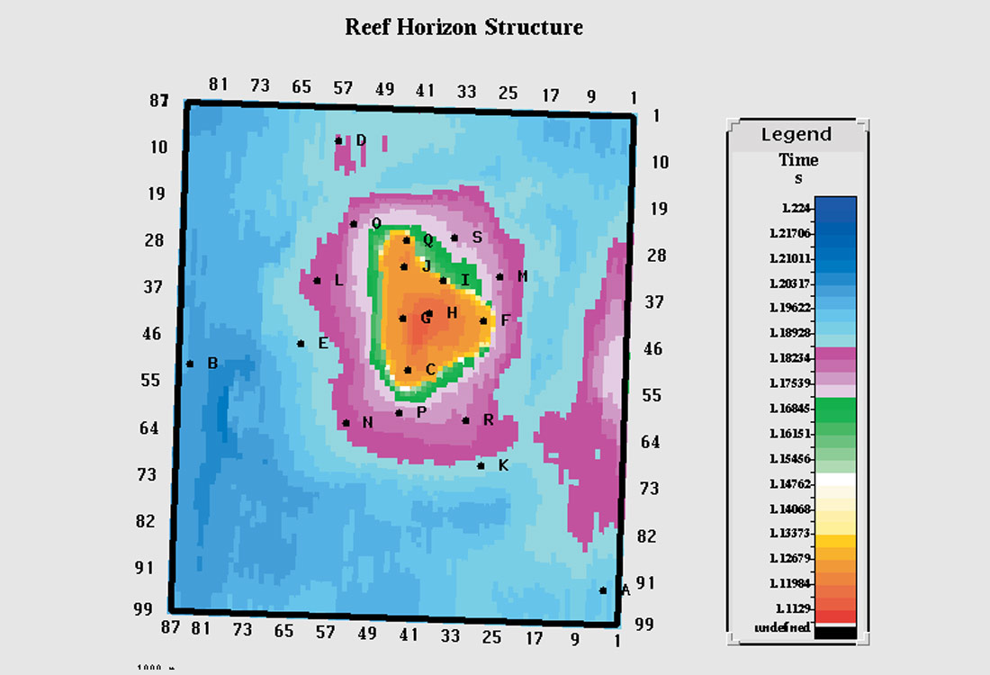
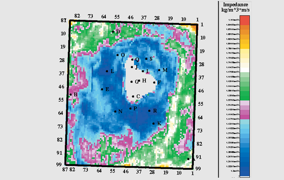
The geology is that of a Western Canadian Devonian reef. Figure 1 shows the reef structure and the locations of the wells. The width of the main build-up is about 1 km. Surrounding the main reef is a porous apron which, away from the reef core interfingers with tighter facies. A lateral salt is present which is dissolved close to the main reef build-up. There were several episodes of dissolution. Some were compensated by the basin material and some were not. This has had some influence in the small scale structure of the off-reef events. The off-reef basin facies are dolomitic and contain thin anhydrites which onlap against the reef. The considerable velocity contrast between the porous reef core and the high impedance offreef facies has resulted in push-down of the reef platform and lower horizons. Other major reflectors are a shale-carbonate transition above the reef and a second deeper laterally continuous salt under the reef platform.

Methodology

Creating an Earth Model

The first step in model building is to design the structure. This is done by providing two pieces of information - the interpreted horizons and the model “framework”. The framework, in the form of a spreadsheet, describes the ordering of the horizons in space and time and their behaviour at faults. The horizons, which can include interpreted faults, provide structure information. Together, these form a blueprint for the model. Stratigraphy within the layers is specified as onlap, offlap, reef, channel, etc. The model is completed by populating it with geophysical information, usually input in the form of well log data. We are most interested in impedance since this is needed to complete the low frequency portion of the seismic inversion.

The logs are usually provided in depth and the horizons in time. Thus it is necessary to create a time-depth transformation if these two pieces of information are to be rationalized. Input sonic logs are integrated, hung on an input time datum (one of the input horizons) and drift-corrected to tie the time horizons. Upon completion, the model exists in both time and depth and time-to-depth and depth-to-time transformations are possible. Interpolation of the input log information between wells is done along layers, respecting both stratigraphy and faults. One of several simple schemes such as linear interpolation or kriging is generally used. This is more than adequate for the task of computing a low frequency background model for the inversion.

Constrained Sparse Spike Inversion

Constrained sparse spike inversion models the input seismic data as the convolution of the seismic wavelet with a reflection coefficient series. Wavelet analysis is accomplished by computing a filter which best shapes the well log reflection coefficients to the input seismic at the well locations. Because the seismic wavelet is bandlimited, the problem is non-unique. There are many reflection coefficient series which, when convolved with the seismic wavelet, reproduce the input seismic to an arbitrary degree of accuracy. To find the best geophysical and geological solution from the large number of available mathematical solutions, we must impose other conditions. These are provided by geophysical constraints which describe how the impedance can vary laterally away from the wells. A “fairway” of allowed impedances is defined, which limits the variability of inversion impedances and automatically rejects many good mathematical solutions which are geophysically or geologically unjustifiable. The impedance fairway is interpolated throughout the model along the model horizons, in turn making the seismic constraints somewhat dependent on the model.

The final step in the seismic inversion is to define a transition frequency, below which information in the final inversion is provided by the model. The model can be computed using logs from a single well or many, depending upon the circumstances. Above the transition frequency, information in the inversion comes from the constrained sparse spike output as described above.

Results

Data

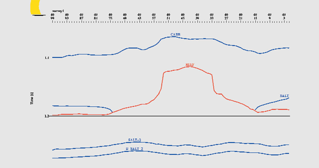
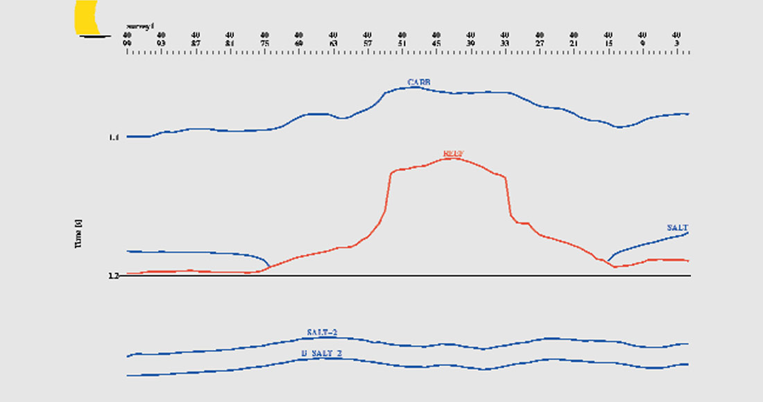
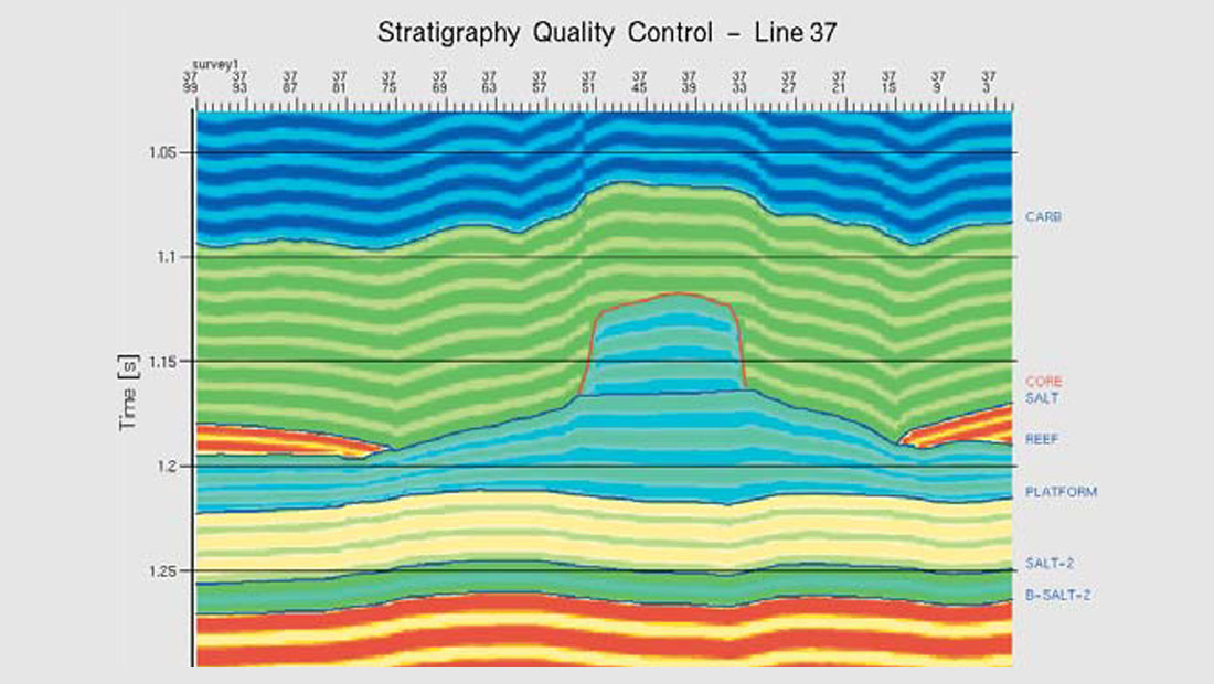
The project data consisted of 100 lines, each with 90 CMP’s. The bin size was 40 * 40 m. Time migration before stack had been done and care taken to preserve true amplitudes. Nineteen vertical wells, each with sonic and density logs were used and porosity logs were available for many. Several horizontal wells were also available for use as quality control. The key interpreted horizon was the “Reef” event which was picked along the top of the build-up until the salt was encountered whereupon the salt base was followed. Other key horizons were the shale carbonate interface above the reef, the reef platform and the tops of both salts. The interpreted horizons along the key line 40 are shown in Figure 2.

Modelling Using Only an Off-Reef Well

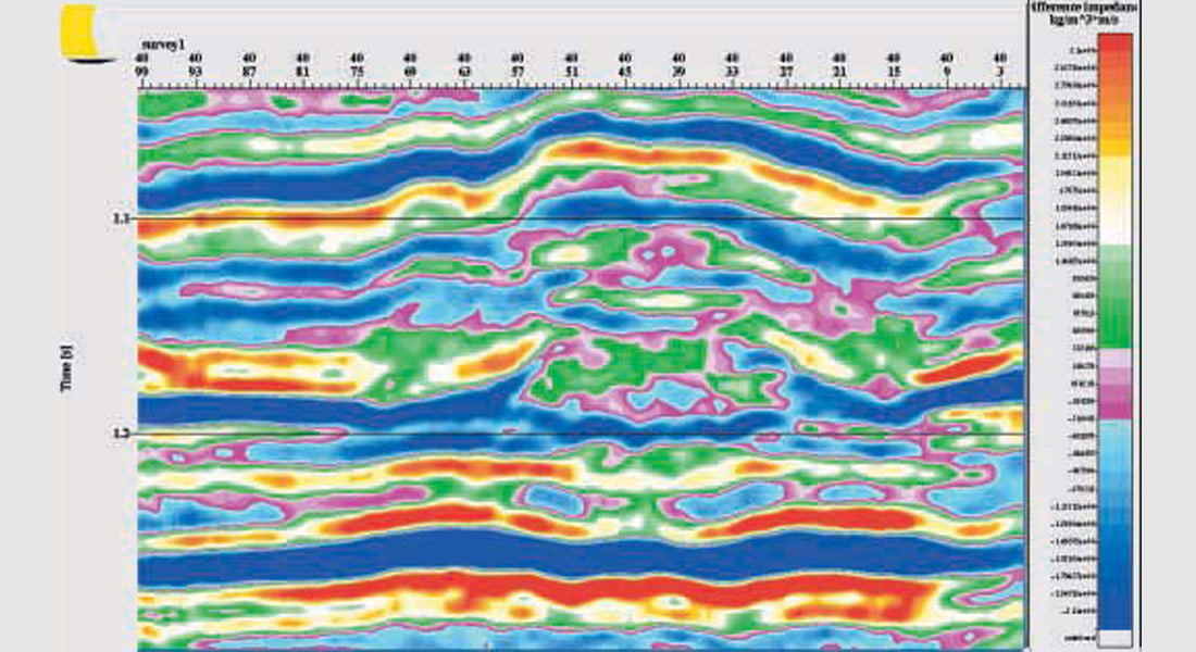
Initially, we do not assume a knowledge of either the reef or even its event horizon. We use only the distant off-reef well, “A”. This well encountered salt and platform facies with no reef build-up at all. The salt in this initial model was allowed to collapse, not against a reef but erroneously against the regional platform. With this incomplete information, a 3D impedance model was constructed, a line through which is shown in Figure 3.

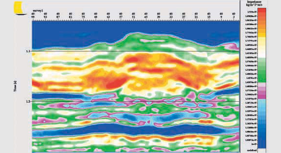
The wavelet was estimated from a comparison of the well “A” impedance log and seismic traces near the “A” location. After an inspection of the amplitude spectrum of the wavelet, the transition frequency was set at 10 Hz where the wavelet power rolled off. In the final inversion, frequencies below the transition frequency are taken from the model. We also produced a relative inversion containing only frequencies at and above the transition frequency. Sections along the key line 40 are shown in Figures 4 and 5 for the relative and full inversions, respectively. Note that the relative inversion does indicate a build-up and evidence of local low impedances. The high impedance anhydrites lapping up against the reef are strong indicators of structure. The build-up itself would certainly be evident from the seismic reflection data too, although the interpretation of the low impedance layers would be less so. Even though the reef has been placed in an incorrect off-reef geologic setting, the existence of anomalous activity in the full inversion (Figure 5) is still evident.

Modelling using the Off-Reef Well and One On-Reef Well

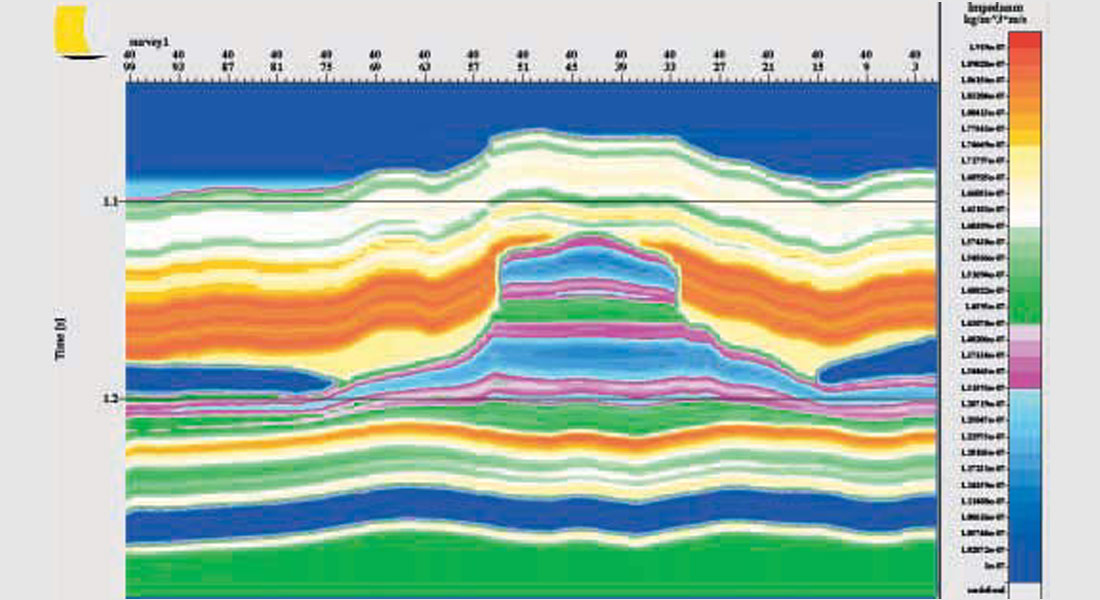
Given the above results, an explorationist might choose to hypothesize the existence of a reef, interpret a potential reef horizon and then place a pseudo well within it. The pseudo well would contain reef-like impedances. The model could then be re-built, and the inversion re-run to test this reef hypothesis. Geologic settings notwithstanding, most geophysicists would be drawn to the activity between CMP’s 42 and 52 and indeed well “G” was drilled nearby. We now assume existence of each of the wells “A” and “G”, and then re-build the model and re-compute the inversion. The existence of a reef horizon is also now assumed. We used the same reef horizon as shown in Figure 2. In the early stages of development, it might be more uncertain. This will not affect our conclusions. We expect to fine tune the horizons as new wells become available, thus uniquely positioning key layers in time and space. The updated model is shown in Figure 6. Since only a single well lies within the reef core, the on-reef impedance is laterally homogeneous except for structure effects. The corresponding full and relative inversions are shown in Figures 7 and 8. Now the geologic setting has been rendered with considerable accuracy. This with just two wells. The meaning of the fine seismic detail has been made clear and more reliable judgements about the locations of future wells made. In this way sweet spots within the reef can be detected and exploited.

We note that the relative inversions in Figures 8 and 4 are virtually identical. They would only have been different if new well information had revised the expectation of the range of impedance values in the region of interest. Then, the constraint fairway defining the constrained sparse spike solution space would have been updated. Other differences could have resulted from re-estimating the wavelet using the “G” impedance log. We did not do this since well “A” was one of the few to encounter the lateral salt. This resulted in a highly characteristic impedance log and less non-uniqueness in the estimation of the wavelet.

Modelling using Well “A” and All the Reef Wells

We now assume some passage of time. In our exploration model several on-reef wells have been drilled. After each, the reef horizon was re-interpreted and new impedance logs were used to upgrade the model. Subsequent inversions were used as an aid in determining future drilling locations. Eventually, interest was directed to the apron facies. Were there regions of enhanced porosity in the apron?

To answer these types of questions, apron impedance maps can be made. This was done here, by copying the reef apron event below itself, re-building the model and then measuring the average impedance in the layer between the reef and copied-reef horizons. Since this layer is conformable with the apron horizon, the average of the inversion within it is a measure of the lateral variation in average apron impedance. We first mapped the inversion constrained by a model containing logs from well “A” plus all the on-reef wells. Figure 9 is this map for a sub-apron layer 4 ms thick, starting at the Reef event. Apparently, regions of low impedance surround the reef. However, on-reef wells have little to say about the apron facies. Except for some knowledge of structure, we have essentially returned to our single-well scenario. Furthermore, that single well (“A”) did not encounter near-reef apron facies.

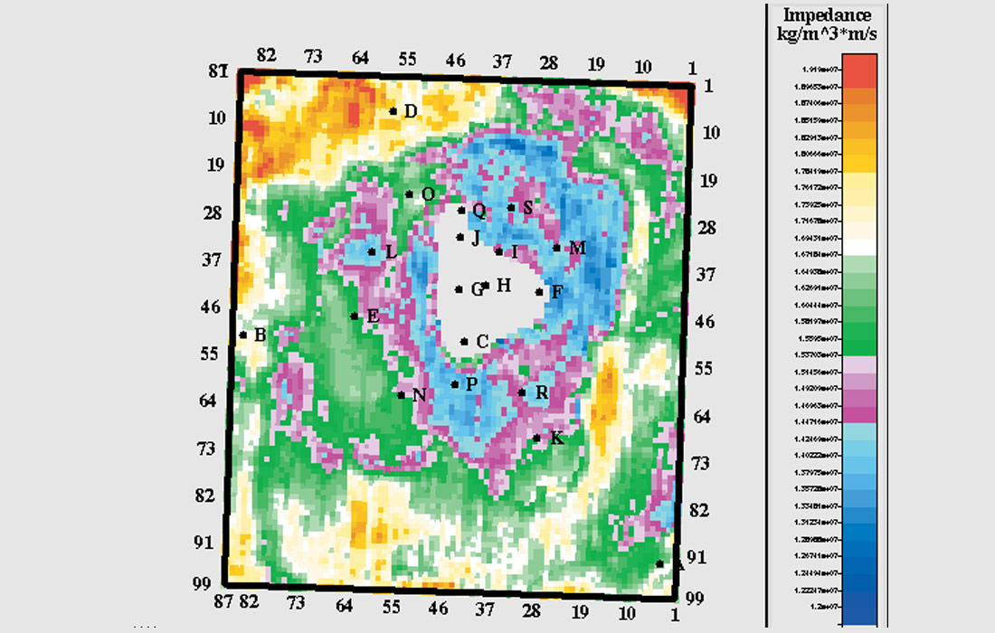
Rather than beginning to add wells one at a time, we look ahead to the present day mature environment and compute a comparable map for an inversion computed from all the wells. It is shown in Figure 10. Porosity development is evident to the south below well P, to the west at well L and to the north and northwest. The good porosity near the reef core is in agreement with horizontal well observations. By comparing Figures 9 and 10, it can be seen that the addition of off-reef wells has added information and highlighted the windward north east as the most prospective area. It is true that we cannot know the low frequency component of the impedance precisely until a well is drilled. But as more wells are drilled in the project area, the model can be upgraded and confidence increased.

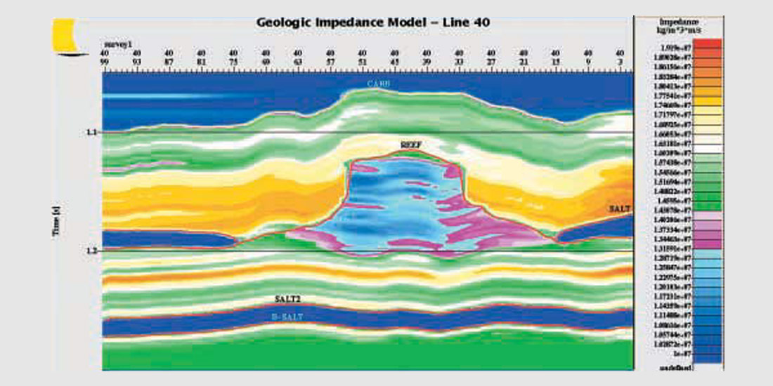
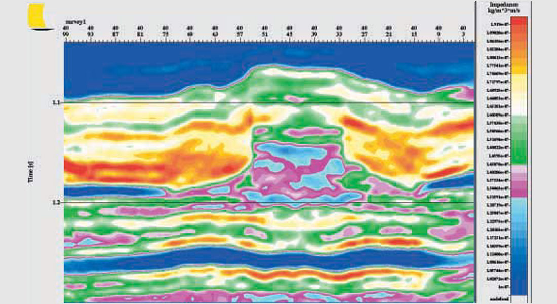
For completeness, we have shown in Figure 11 the model framework corresponding to a section through the final 3D model. The broad colours are meant to indicate the layer boundaries. The structure of the finer banding internal to each layer is indicative of the stratigraphy. In most layers, the stratigraphy is conformable with the bounding horizons. Exceptions are the Salt layer which is conformable only with its upper boundary and the reef interior which has been defined to respect both the reef structure and the observed push-down. Figure 12 is the same section through the final impedance model. Lateral variations in impedance arise from both structural and stratigraphic effects. At CMP’s where no log is present, nearby logs were stretched or squeezed on a layer-by-layer basis to account for structure and then subjected to a weighted average to arrive at the model impedance. A simple distance-weighted average sufficed although the weights could have been set arbitrarily as required. The final full inversion using all the wells is shown in Figure 13.

Conclusions and Discussion

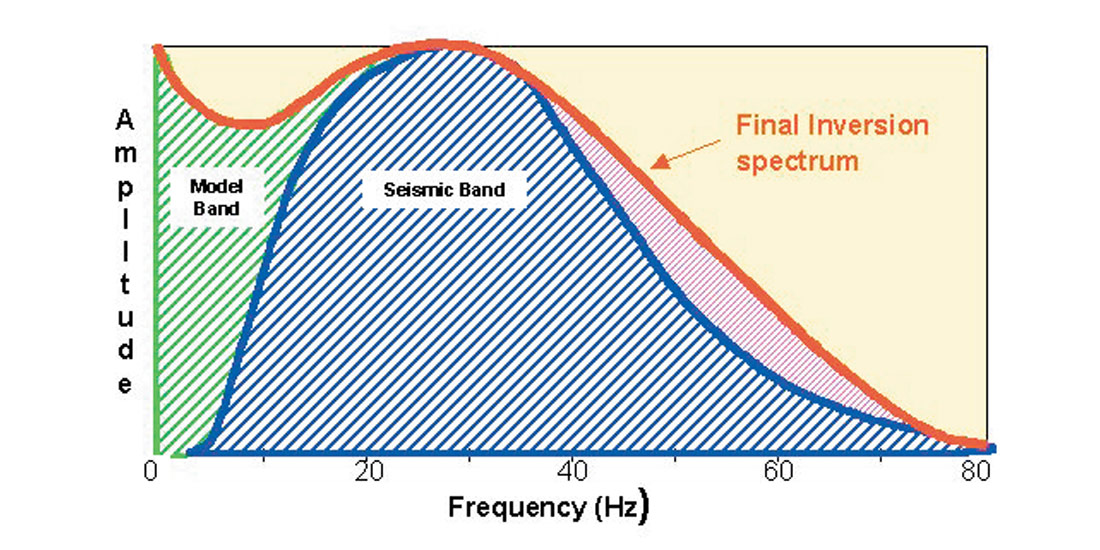
We have demonstrated that seismic inversion can be useful in both exploration and production environments. The high frequency seismic band component of the inversion remains remarkably constant from rank exploration to mature production. The reason for this is simple. The inversion result is constrained only to lie within the impedance constraint boundaries. It is not constrained to be similar to any particular impedance log, even when inverting at that CMP corresponding to the well location. Therefore, a comparison with log impedances is a very powerful QC tool. Significant changes could only result from an improvement and general tightening of the sparse spike constraints and re-estimation of the wavelet. These can be implemented as more wells are drilled and there is a better understanding of the expected range of impedances. The model and the full inversion are dramatically improved when wells have been drilled through all representative facies. In this case, only two wells were necessary to define the basic geology. As off-reef wells were made available, their contributions to the net porosity could be accounted for and regions of enhanced porosity located. It is not always possible that extensive drilling will have resulted in a thorough a priori understanding of the play. But when such knowledge is available, it should be used to build an accurate and detailed model. We have used the abundance of wells not to force the answer in the seismic band but to improve our model and the knowledge of the low frequencies which we extract from it. This idea is illustrated in Figure 14.

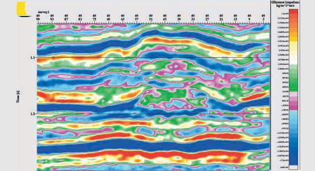
It is perhaps worth emphasizing the importance of formally computing both the relative and full inversions explicitly. Whether the play in question is new or mature, there is always the danger of a misinterpretation. The relative inversion is mostly immune to this condition. When horizons are at all suspect, the constraints are simply relaxed a little. It is a different story in the case of the full inversion. Misinterpretations will change the model and the way in which the low frequencies contribute. Given the large amount of power in the low frequencies of logs and inversions, the effects can be dramatic (compare Figure 5 and 7). Fortunately, these problems can be easily ameliorated or a least risked by a simple comparison of the relative and full inversions.

Acknowledgements

The authors gratefully acknowledge Husky Oil Ltd. and Mobil Oil Canada for their generous donation of these data.