Classification of microseismic events via principal component analysis of trace statistics

Abstract

Prior to microseismic hypocenter location, an event-classification technique must be used to identify “good” events warranting further investigation from “noise” events that are generally not of interest. A passive-seismic monitoring system may record tens or hundreds of thousands of microseismic traces daily, so the event classification method must be precise and automatic (and preferably fast enough to be applicable before event recording). Using microseismic data from Cold Lake, Alberta, provided by Imperial Oil Limited, we determined that three simple statistics, derivable from individual microseismic traces, gave the most robust differentiation between “noise” events and “good” events (classified manually beforehand). We developed a classification scheme based on principal component analysis of the three statistics to further enhance classification performance. Testing of the method implemented in MATLAB code yielded classification accuracies between 90% and 99.5% over a wide range of data files.

Introduction

Imperial Oil Limited is involved in oil sands production at Cold Lake, Alberta, Canada. Hydrocarbon production comes from the Clearwater Formation. This producing formation is mostly sandstone and is buried over 400m deep at Cold Lake. The bitumen contained within it has an American Petroleum Institute (API) gravity index of approximately 8° to 9°. Cyclic steam stimulation (CSS) is required to extract the viscous bitumen (Tan, 2007). CSS creates pressures and temperatures of approximately 320°C and 11 MPa in the formation. Mechanical issues in producing wells such as cement cracks or casing failures can result from the high pressures and temperatures associated with CSS.

If undetected, these production issues could result in large cleanup costs, in addition to potential legal implications. A microseismic earthquake with its focus near the damaged area is created when such a mechanical breakage occurs. Imperial Oil Limited operates a passive seismic monitoring system at Cold Lake to proactively detect these microseisms. Maxwell and Urbancic (2001) give a discussion on passive seismic monitoring in instrumented oil fields.

The passive seismic monitoring system implemented at Cold Lake is present on approximately 75 production pads. Each pad has a centrally located monitoring well that records ground vibrations (including microseisms). The monitoring well is instrumented by a down-hole array of five or eight 3- component (3-C) geophone sondes connected to seismic recorders at the surface (Tan et al., 2006). Seismic recorders listen for discrete seismic events and store them as microseismic event files to disk for later review. For an array of five or eight geophones, these digital event files contain fifteen or twenty-four traces that display about 1.4s of microseismic activity recorded by the 3-C geophone sondes. Vendorsupplied event-classification software analyzes each created microseismic file and assigns a classification. If a file is classified as “good”, this indicates that the software has decided that the event file warrants further investigation. Conversely, if a file is classified as “noise”, it is supposedly an event that is not of interest (Tan et al., 2006; Tan, 2007).

Approximately 99% of all detected events are noise. Examples of “good” events worth further investigation include cement cracks around the casing in the wells, and casing failures. Examples of noise events include noise created by pump rods and passing vehicles. When a “good” event is automatically detected followed by manual confirmation, an attempt is made to locate its hypocenter (that is, its point of origin).

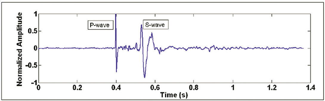
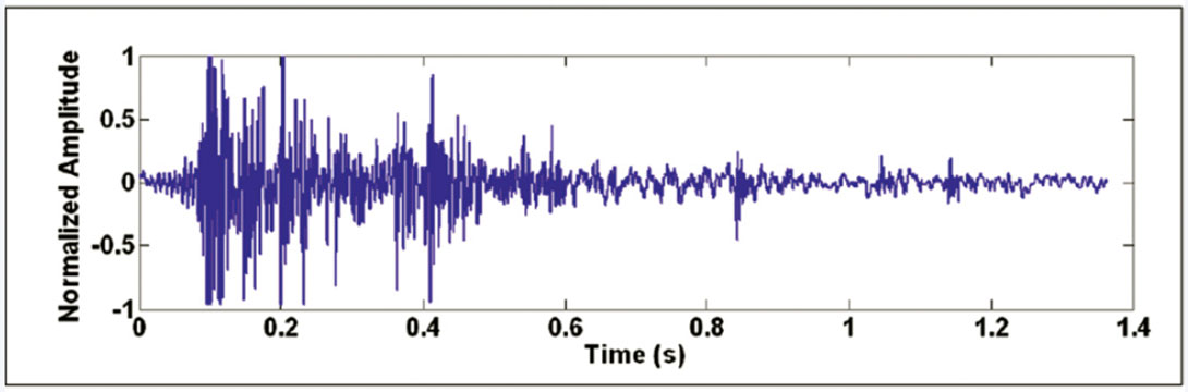
Figure 1 shows an example of a “good” event from the Cold Lake dataset, with P- and S-wave arrivals indicated. Empirically, it can be determined that this event is “good” due to the distinct and impulsive P- and S-wave arrivals. Note the decrease in frequency of the S-wave arrival compared to the P-wave. Figure 2 shows an example noise event; it is generally random and does not follow deterministic properties. The microseismic trace shown on Figure 1 or 2 has been processed to remove any DC offset and normalized by the largest data value on the trace. Each trace is 4096 samples long and is digitized at 3000 samples per second.

Standard event-file classification based on signal-to-noise ratios and STA/LTA ratios have been applied to events recorded by the Cold Lake passive-seismic monitoring system. The standard scheme has been known to misclassify a large portion of recorded events. This has resulted in many noise events being incorrectly identified as “good” events, often referred to as “false positives”. Manual investigation of misclassified files can become very costly and time-consuming.

In this paper, we will describe the development of automatic and robust microseismic signal analysis algorithms capable of precisely classifying tens of thousands of microseismic event files generated daily by the passive-seismic monitoring systems.

Trace Statistics

Compared to noise traces, “good” microseismic traces generally contain lower signal variance, higher central data distribution, more frequent oscillations, and greater signed amplitude differences between adjacent time-series data points. Statistical analysis classification algorithms were developed based on these observations (Tan, 2007).

Threshold algorithm

Chebyshev’s inequality is given as

Pr(|x –E[x]| ≥ a) ≤ var[x]/a²

(e.g., Suhov and Kelbert, 2005), where x is a random variable with expected value E[x] and variance var[x], a is a strictly positive constant, and “Pr( )” is the probability. For a zero-mean microseismic signal, x refers to the time series data points, E[x] = 0, and var[x] is the microseismic signal variance.

Chebyshev’s inequality states that a larger dataset variance corresponds to an increase in the expected maximum number of data points lying outside a mean-centered window of width 2^a. We used this fact to develop a simple threshold algorithm for classifying a microseismogram, or a file of microseismograms. Define an amplitude window (-a, +a) centered at the mean (adjusted to be zero, if need be) of a microseismic trace. The threshold algorithm simply determines the fraction of time series data points with amplitudes that lie outside the range (-a, +a). This fraction can then be used for microseismic signal classification. For example, using a = .006, the normalized “good” trace in Figure 1 has 20.8% of its time series data points outside the window, while the normalized noise trace in Figure 2 has 68.2% outlying data points.

Histogram algorithm

The signed amplitude distribution of “good” traces tended to be more heavily concentrated near the time axis than noise traces, as can be seen in the “good” and noise traces on Figures 1 and 2, respectively. One tool that can be used to examine and quantify data distribution is a histogram.

Let d_max and d_min denote the possible maximum and minimum values in a microseismogram. For a normalized zero-mean trace, these values are +1 and –1, respectively. Define 99 histogram bins each with a bin width of .02 covering the range (-1.00, +1.00). Then, fill each bin with the fractional number of data points with amplitudes falling within the bin limits (the fractional numbers for all bins must sum up close to 1.000). Plot the distribution of amplitude values as a histogram. Figures 3 and 4 show histogram plots corresponding to the “good” and noise traces depicted on Figures 1 and 2.

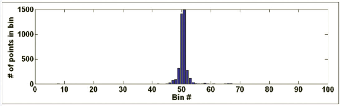
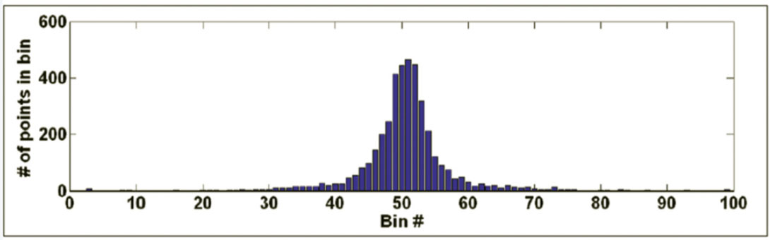
After histogram generation, the value recorded in the central bin can be examined for microseismic signal classification. For the “good” trace depicted on Figure 1, 34.6% of its time series data points lie in the 50th bin (i.e., points having amplitudes between –.01 and +.01). For the noise trace on Figure 2, only 10.7% of its points fall in this range. Note the higher central concentration of data points for the data point distribution of the “good” trace, as compared to the noise trace, which shows a data distribution with a wider half-width.

Specialized Zero-Crossing Count algorithm

Microseismic traces determined manually to be “noise” tended to oscillate more frequently about the time axis. Additionally, the signed amplitude differences between adjacent time-series data points were generally greater for “noise” microseismic traces compared to “good” traces. In other words, compared to “noise” traces, “good” traces often have less sporadic sequential timeseries behaviour about its mean.

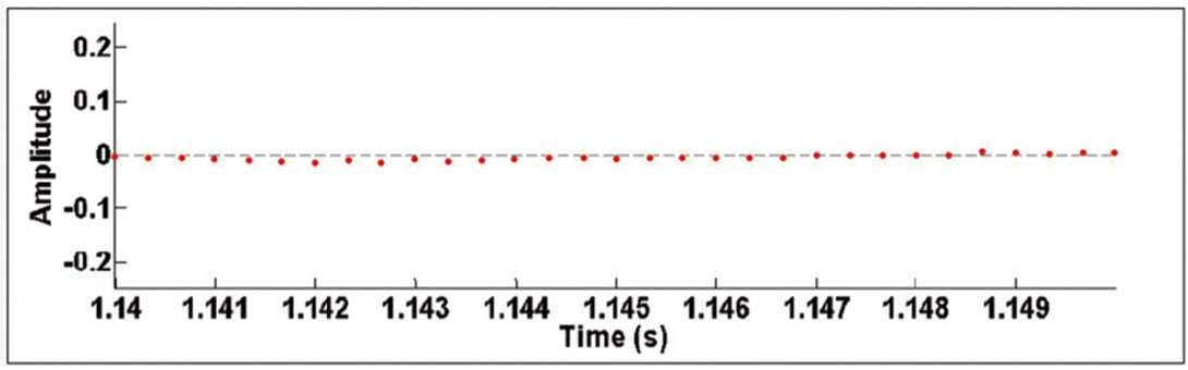
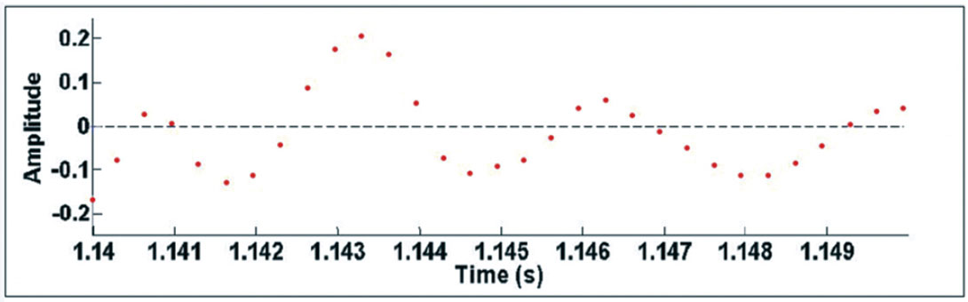
To illustrate the above observations, parts of the “good” and “noise” traces on Figures 1 and 2 are plotted as discrete time-series on Figures 5 and 6. A very fine time interval from 1.14s to 1.15s is used in these figures to accentuate the differences in frequency and amplitude of oscillations on “good” and “noise” traces. Note that on Figure 6, corresponding to the “noise” trace, there are more instances where adjacent data points have opposite signs compared to the “good” trace on Figure 5. That is, “good” traces oscillate less than “noise” traces, and the amplitudes of the oscillations are much less. Based on these observations, the “Specialized Zero-Crossing Count” algorithm was developed.

Define a window that exists in the signed-amplitude range (-z, +z). First, set all the time-series data points that fall within this range to zero. Essentially, this zeroing step removes low-amplitude noise. As the signed amplitudes of adjacent time-series data points in microseismic “noise” signals generally vary to greater degrees compared to “good” traces, this zeroing step will tend to preserve polarity reversals (sign changes) in adjacent data points on “noise” traces, but eliminate many of these polarity reversals on “good” traces. Thus, this step helps to accentuate the discrepancy between “good” and noise traces and improve classification accuracy.

After the zeroing step is applied, count the total number of valid polarity reversals between adjacent data points, and divide by the total number of trace data points to obtain a fractional measurement. A valid polarity reversal corresponds to adjacent data points changing from a strictly positive to a strictly negative value, or vice versa.

With the zeroing step applied for z = 0.01, the “good” trace on Figure 1 had only one valid polarity reversal out of 4096 total data points, corresponding to a percentage of 0.0244%. On the other hand, the “noise” trace on Figure 2 had 298 valid polarity reversals, for a percentage of 7.28%.

To illustrate the value of applying the zeroing step to eliminate low-amplitude noise present in the time series, consider the case where it is omitted. If this zeroing step is not applied, the “good” trace on Figure 1 would have 302 polarity reversals out of 4096 points (7.37%), while the “noise” trace on Figure 2 would have 550 polarity reversals (13.43%). Thus, omitting the zeroing step, only 1.82 times more polarity reversals would be seen in the “noise” trace compared to the “good” trace. With the zeroing step applied, 298 times more polarity reversals are seen in the “noise” trace compared to the “good” trace.

Principal Component Analysis

The outputs from these three statistical algorithms can be used for accurate microseismic file classification. As it stands, we must use three statistical outputs to differentiate between “good” files and “noise” files. We can simplify the classification decisionmaking if we combine the information in the three statistics into a single parameter. We do this by applying principal component analysis (Jackson, 1991; Shlens, 2009).

Principal component analysis (PCA) is a linear technique that transforms a dataset with N variables so that the data can be represented by N orthogonal basis vectors (principal components). When this is done, the data can be projected onto the first principal component which has the highest variance and thus best characterize the dataset. PCA was applied to the outputs of the three statistical algorithms to simplify and improve classification accuracy.

To illustrate the application of PCA to microseismic file classification, a diverse example test dataset of 540 microseismic files from 28 different production pads was used. The correct file classification was known, as these files had been manually classified as “good” or “noise”.

We defined a 3 x 540 matrix A whose rows correspond to the three statistics, and whose columns correspond to different microseismic files. The normalized results from the Threshold, Histogram, and Specialized Zero-Crossing Count algorithms were placed in the first, second, and third rows of A, respectively. More specifically, each row element of A was filled with the normalized average algorithm outputs corresponding to the three traces in a microseismic file that have the strongest “good” characteristics. For example, the element a₁₅ is the normalized average fraction of data points lying outside a predefined window (Threshold algorithm) for the three traces in the fifth microseismic file having the lowest fraction of outlying points.

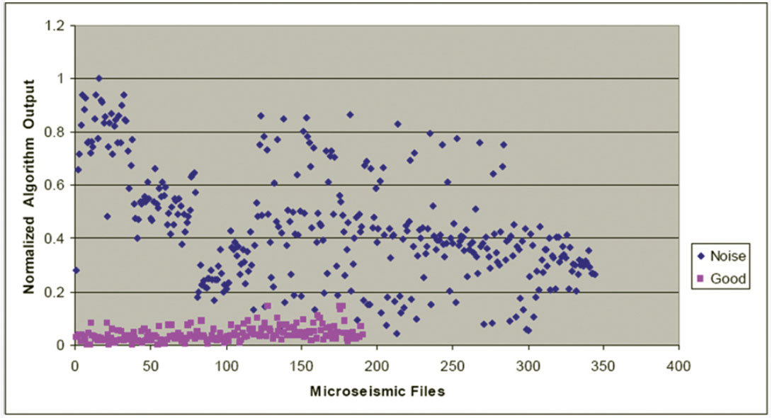
Figures 7, 8, and 9 show plots of normalized algorithm measurements contained in the first, second, and third rows of A, respectively. There are 540 plotted points corresponding to the 540 files used in the analysis. Figure 7 shows the normalized Threshold algorithm output, which corresponds to the normalized fraction of data points with normalized amplitudes outside the range (- 0.006, +0.006). Each pink square represents the Threshold statistic from a manually confirmed “good” file, while each blue diamond corresponds to the Threshold statistic from a manually confirmed “noise” file. Ideally, with this statistic, there would be no overlap between known “good” and noise files. On Figure 7, there is reasonable vertical separation (with some overlap) between the “good” and “noise” files.

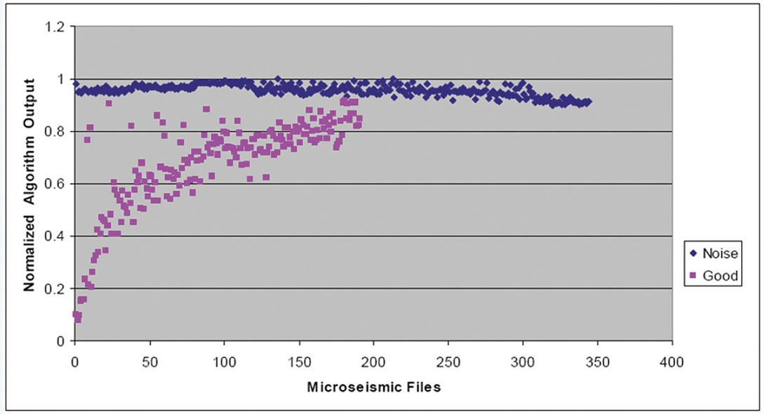
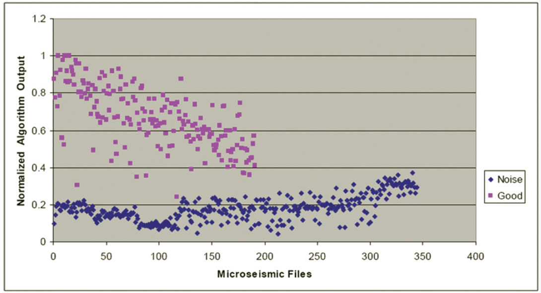
Figure 8 shows the normalized Histogram algorithm output (i.e., the normalized fraction of points that are contained in the 50th data bin, or the number of points with amplitudes closest to zero) for the 540 files. Reasonable separation is seen between “good” and noise outputs; however, some overlap still exists.

Figure 9 shows the normalized Zero-Crossing Count algorithm output (i.e., the normalized fraction of signal polarity reversals after low-amplitude noise is removed). In this example, data points with a magnitude less than 0.006 were set to zero. There is good separation between “good” and “noise” outputs, with some minor overlap between “good” files and “noise” files.

We wanted to reduce the overlap between known “good” and “noise” files to obtain better microseismic file classification. This was achieved by projecting the measured data shown in Figures 7 to 9 onto the dataset’s principal components. To find the principal components of the dataset, we used the fact that the principal components are equivalent to the unit-length eigenvectors of the dataset’s covariance matrix (Shlens, 2009).

The measurement matrix A has three rows and 540 columns. After normalizing each row by its maximum value and meancorrecting the row to zero, we find the symmetric 3 x 3 covariance matrix C of the dataset:

where n = number of columns of A. The first, second, and third rows of C contain covariance values that involve the Threshold, Histogram, and Specialized Zero-Crossing Count algorithm outputs, respectively.

For this symmetrical 3 x 3 covariance matrix, there will be three corresponding unit-length orthogonal eigenvectors each representing a single principal component of the dataset. The eigenvalue of each eigenvector is equivalent to the data variance when projected onto the eigenvector. The eigenvector with the largest eigenvalue represents the first principal component of the dataset and is orientated in the direction of maximum data variance. The eigenvector with the second largest corresponding eigenvalue represents the second principal component of the dataset, and so on. After mean-correction, the normalized measurement data contained in the matrix A was projected onto the principal components of this example dataset containing 540 microseismic files. Figures 10, 11, and 12 show these data after projection onto the first, second, and third principal components, respectively.

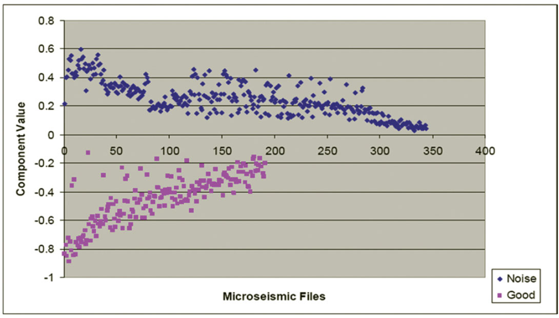
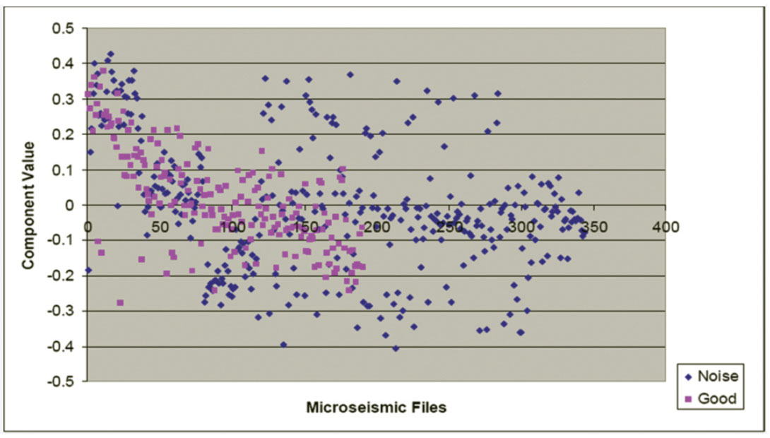
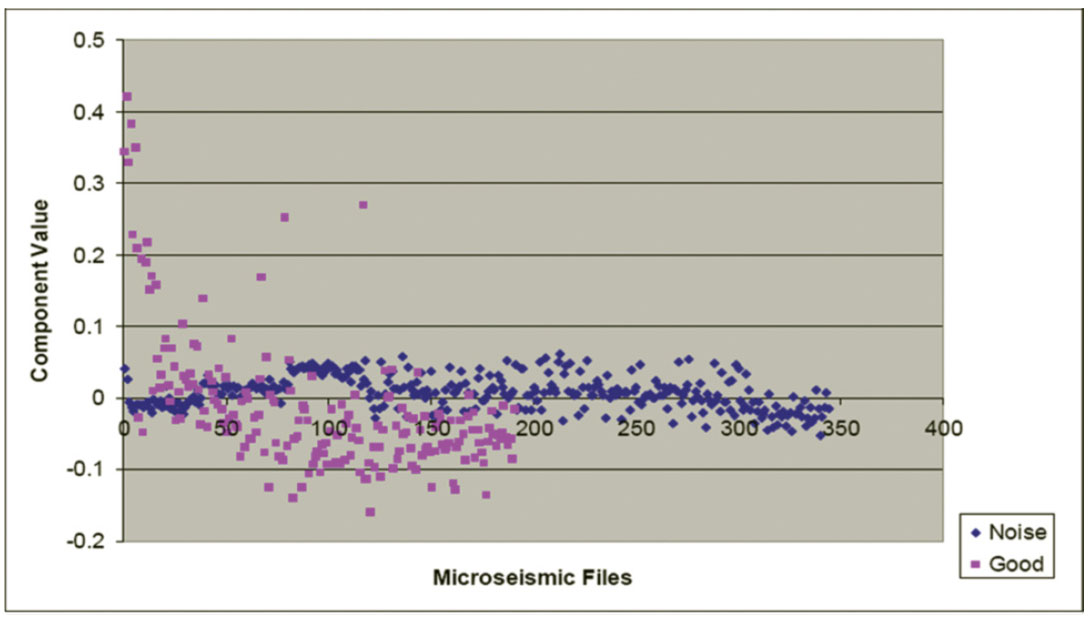
On Figure 10, there is no overlap between the “good” and noise data points, clearly suggesting that applying PCA analysis to file classification would be an improvement over attempting to empirically classify files with the raw statistical measurements shown on Figures 7 to 9. Figures 11 and 12 correspond to noise components in the data, and show no separation between “good” and “noise” files. These principal components therefore are not useful for microseismic file classification. For this dataset, PCA has reduced the effective dimensionality from three to one.

Figure 10 suggests that if the dominant eigenvector resulting from PCA is used for multivariate data reduction, all 540 files from 28 different pads in this specific example dataset could be classified to perfect accuracy. This obviously will not always be the case for all datasets, but applying PCA does result in improved classification accuracy over simply observing individual algorithm outputs for classification.

The principal components derived using the 540 files from the 28 pads can be used to classify a new file of microseismograms. The three statistics are calculated for the new file. The values used to mean-correct and normalize the rows of the original 3 by 540 matrix A are applied to the three statistics for the new file. The corrected statistics form a vector of length 3 which is then projected onto the first principal component to yield a single parameter. This parameter, when plotted on Figure 10, classifies the file as “good” or noise.

Conclusions

Threshold, Histogram, and Specialized Zero Crossing algorithms were developed to generate three simple statistics from microseismic traces. These statistics were effective in differentiating “good” data files from “noise” data files recorded by passive seismic monitoring systems in a heavy-oil production facility at Cold Lake, Alberta, Canada. The statistics were based on the observation that, compared to microseismic noise, “good” microseismic signals contained lower signal variance, narrower data distribution, and less sporadic sequential time series behaviour about its mean. In addition to strong classification performance, the statistical analysis algorithms were found to be computationally efficient, a required characteristic if they are to be used for classifying tens of thousands of microseismic files daily.

Our final classification scheme applies principal component analysis to the three simple statistics to further enhance the differentiation between “good” and “noise” files.

Implementation of the scheme in MATLAB code is robust and yields accurate results over diverse datasets without altering any program settings. When applied to a specific dataset where most files originated from five production pads at the Cold Lake site, an accuracy of 99.5% was obtained. Testing on a more diverse dataset with files from 28 different pads yielded a classification accuracy of 98.8%. An exhaustive test on microseismic files from 72 different production pads resulted in a 90% accuracy. In conjunction with our continuing interest in passive seismic monitoring, CREWES will use this classification technique in studies of other large microseismic datasets.

Acknowledgements

We would like to thank the industrial sponsors of CREWES and NSERC for their support of this research. We are also grateful to Colum Keith, Richard Smith, and Sophia Follick from Imperial Oil Limited; they provided us with microseismic data, performed a wide variety of testing on the developed program, and consistently gave valuable feedback.