Changing Visualization Technology

Introduction

Consider this scenario: you are given a 3-D survey known to contain channel sands within a prospective interval. Your job is to quickly identify potentially interesting prospects. To accomplish this quickly, which view would you prefer?

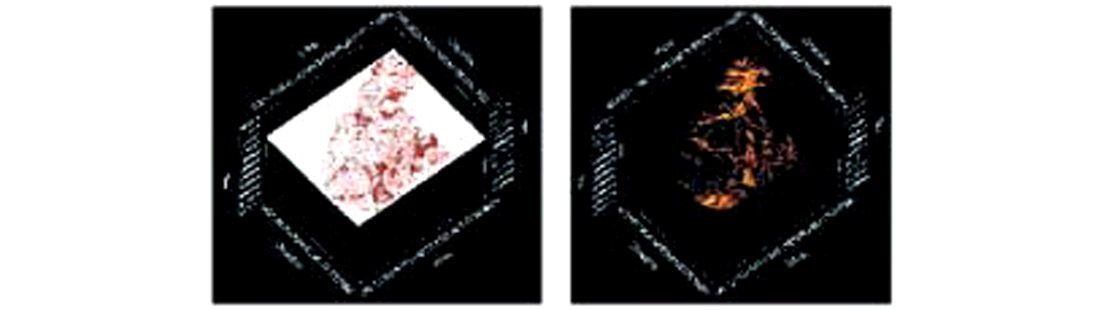
The view on the left is a typical time slice view created by polygon representation. The view on the right is a voxel view created by volume rendering. Technology changes in the late seventies made the left view possible. Technology changes in the late eighties made the right view possible. Recent changes in PC hardware are making volume rendering readily accessible to the average geoscientist.

From Vector to Raster

During the sixties and seventies, graphic visualization was confined to vector drawing of objects. With this technology, only continuous line segments added together are used to build up images. The screen is refreshed by redrawing all the objects contained in a display list. Object oriented operations such as translation, rotation, and sizing are easy to accomplish and the continuity of lines guarantees the absence of aliasing. However, this technology cannot shade or color interior areas and is not well-suited to display of sampled data. In addition, as the number of objects in the display list increases, rendering performance decreases.

Since the late seventies raster graphics has replaced vector graphics technology. This technology uses a 2-D frame buffer or raster of pixels to build up the screen image. Individual point rendering allows the coloring and shading of each pixel to create interior texture within displayed objects. Screen refresh is accomplished by repeatedly displaying the frame-buffer on screen. This effectively decouples image generation from screen refresh. Memory and processing requirements are large and constant, which has not presented a problem since the late seventies. Raster graphics is by its very nature sampled display and so is ideal when trying to display sampled data such as seismic and well data.

Raster graphics has been combined with the object-based approach of vector graphics to give us surface graphics familiar to us in our current interpretation workstations (and our playstations at home). This technology employs polygons to represent data. Object oriented operations such as translation, rotation, and sizing are easy to accomplish with the polygons. Seismic data and other earth data are easily displayed in a 3-D view using this technology although performance is affected by the number of polygons in a scene. However, it is important to realize that polygon views are only 3-D surface views. At any particular time only a small portion of the available data is ever displayed.

From 3-D Surface to Volume Graphics

Surface graphics has allowed us to more easily interpret in a 3-D sense by using 3-D surfaces. However, the two images above show clearly the limitation of surface graphics. The world really is a 3-D world and geology is best viewed in a 3-D volume for ease of visualization. However, volume visualization requires large amounts of memory since all data must be held in memory for speed of access.

Volume graphics offers the same benefits as surface graphics, with several advantages. These include constant (but large) memory requirement and insensitivity to scene and object complexity. Because the data is represented as voxels, viewpoint independent information can be precomputed and stored during the voxelization of the data, which is done independently of viewing the data.

Traditionally, volume graphics has only been available on high-end workstations using expensive graphics cards containing texture memory (TRAM). Cost considerations have adversely affected the wide spread adoption of this technology. However, this is about to change with the introduction of new CPU rendering techniques and more powerful PC hardware as described below.

TRAM Visualization Systems

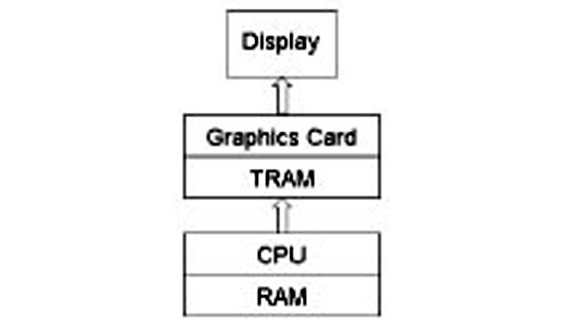
Voxel visualization has been available for more than a decade in the oil and gas industry. Initially, image rendering had to be done using specialized graphics cards with texture memory or TRAM. Even today final rendering and display is often done on the graphics card using older rendering algorithms. Rendering a complete volume of data to create an image must necessarily be extremely fast if it is to appear real time. When rendering occurs on the graphics card, all the data must be passed from memory (RAM) to the graphics card. This requires that the RAM, CPU, and graphics card be together in one location. The hardware and data flow can be diagrammed as follows:

Implicit in the diagram is the volume size limitation inherent in a single CPU system. Maximum RAM size is limited to addressable space. A thirty-two bit operating system such as Windows can address 4 Gb of memory but because of operating system requirements only 2 Gb is readily available for holding data. Future 64-bit PC operating systems will break this limitation. However, this creates another problem because removing the 2 Gb restriction creates a bottleneck between the CPU and the texture memory on the graphics card.

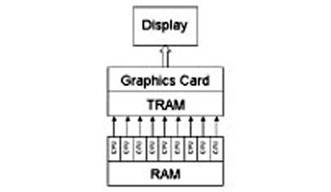
High performance high-end workstations have solved the 2 Gb limitation by a combination of adding CPUs in parallel and adding texture memory. The larger data volumes available require specialized hardware, or graphic pipes, to speed the data transfer between CPU and texture memory. Interestingly, the additional CPUs have not required the data be split up among RAM attached to each CPU. Instead, 64-bit addressing allows each CPU access to all the data held in common memory. This system is diagrammed below.

The large volume voxel visualization using multiple CPUs has found use in visionaria and to a limited extent as stand-alone workstations. Price has been the limiting factor since these workstations can easily cost $500,000 to several million dollars depending on the number of CPUs, number of graphics pipes, and amount of texture memory added to the system.

PC Cluster Technology

Ever increasing PC price performance has recently made PCs an attractive platform for 3-D visualization and interpretation. Today, several software packages for the PC employ CPU rendering algorithms to eliminate the need for special graphics cards. This means 3-D visualization and interpretation can be done on a PC costing under $2,000 (US). In fact, CPU rendering means 3-D visualization and interpretation can even be done on a laptop! However, single CPU software on a PC cannot provide a large data volume solution. Experience indicates a modest volume of 500 Mb of initial (usually amplitude) data can be CPU rendered on a pentium IV machine with acceptable performance. Additional attribute volumes can also be loaded up to the 2 Gb maximum. Larger data volumes require the use of multiple CPUs configured as a PC cluster.

APC cluster provides an elegant solution to the large data volume problem. A typical PC cluster for visualization and interpretation uses either the Linux or Unix operating system. Individual units contain a dual CPU motherboard with 2 Gb of memory. The number of CPUs determines the total amount of data that can be loaded so that large data volumes can be loaded by simply adding more CPUs as required. Currently, cost per CPU is under $2,000 (US) and is dropping rapidly.

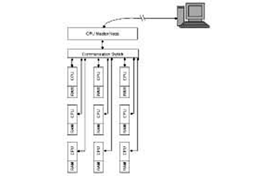
The PC cluster does all the image rendering for voxel visualization and does polygon reduction for any polygon views. The result is that only a small image file is sent to the users workstation, typically a Windows PC. The cluster and viewing screen need not be in close proximity. In fact, visualization has been done across the Atlantic Ocean via the internet with a cluster in the US and a receiving PC in Europe. The PC cluster and viewing workstation can be diagrammed as below.

This configuration provides the power of a super computer for the price of a few PCs. It provides a flexible system that can be expanded or rearranged as required. Maintenance is readily available and inexpensive so cost of ownership is low. Thus, volume visualization has become affordable for the average geoscientist.

Do You Have Large Volumes?

Start with a moderate size dataset, perhaps 300 Mb. This easily fits on your current workstation. However, a typical workflow never uses only one volume. Let's load near and far trace volumes (or P and G cubes if we have them). From this we create a new cube highlighting AVO anomalies. Next, we create a coherence cube to highlight faulting and then an AGC cube to highlight structure. Finally, we want an acoustic impedance cube to highlight interesting formations. Our one 300 Mb dataset has now become seven cubes taking up over 2 Gb of memory. Holding this amount of data in memory and using volume visualization techniques will decrease cycle time, increase our confidence in our analysis, and decrease risk-all desirable results.