Central Alberta Aggregate Study

Abstract

An OhmMapper apparent resistivity survey was undertaken at a site in central Alberta to identify and delineate an aggregate deposit. The results show that the apparent resistivity method has defined the lateral and vertical extent of the main aggregate zone as well as several smaller high-resistivity regions on the periphery of the survey area that may be associated with smaller pockets of coarse-grained material. The system applied to the survey, i.e. OhmMapper, has proven to be a fast, easy and cost-effective technique to obtain both lateral and vertical extents of the economically viable aggregates.

Introduction

Aggregates generally refer to deposits of sand and gravel, coarse-grained materials that may be distinguished by their high bulk resistivity. Sands and gravels are used in a variety of infrastructure projects including roads, foundations, bridges, drill pads, etc. and constitute an essential mineral resource in their own right. While the unit price of aggregates is generally low ($5.79/tonne according to a 2007 resource study published by the Alberta Energy and Utilities Board (Edwards and Budney, 2006)), transportation and haulage costs can vary widely, increasing with the distance between the construction site and the pit. Therefore, locating viable gravel deposits adjacent to proposed infrastructure construction will reduce costs associated with procurement.

Rather than use traditional electromagnetic (EM) or electrical resistivity (i.e. galvanic electrodes) techniques to identify the presence of coarse-grained material at the present survey area, the OhmMapper resistivity mapping system was selected to carry out the investigation. Conventional electrical imaging methods may be used but introduce practical concerns such as electrode insertion into tough, potentially gravelly, ground and lengthened data acquisition times. Electromagnetic methods can, and often are, applied to the problem but lack the vertical resolution required to make volume estimates. The OhmMapper offered both time and cost savings over these methods.

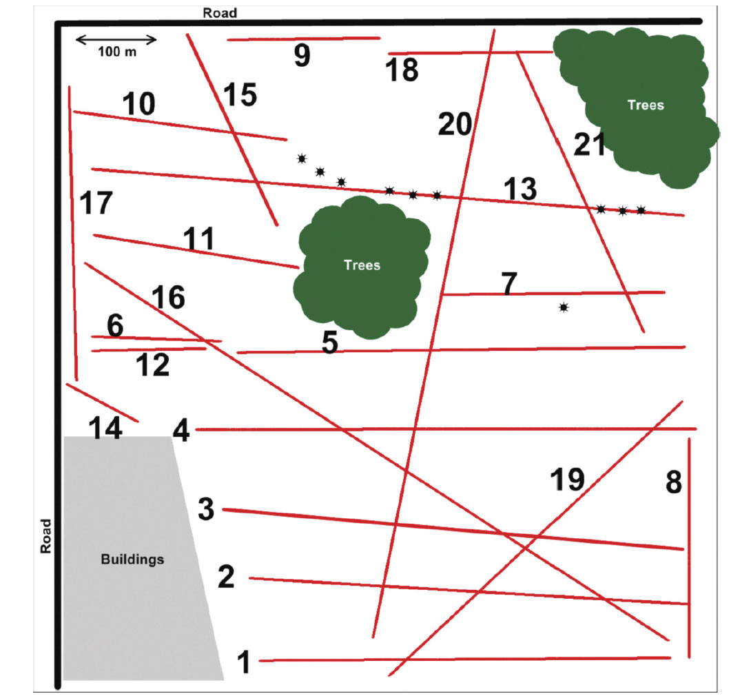
The survey area is located within a quarter section in central Alberta, typically flat-lying pastureland. The survey grid covers an area of 800 x 800 square metres. In the northern portion of the site, the ground is seasonally wet and is populated in areas by small copses of willow. The presence of aggregates was suspected prior to geophysical and geotechnical investigations.

Test pits were excavated after the geophysical survey in an effort to ground-truth the resultant data. Test pitting indicates that the near-surface sediments are comprised of topsoil (generally less than a metre thick) over a thin unit of silt (generally less than 0.25 metres thick) over gravel (over 1 metre in thickness).

Apparent resistivity data were acquired using the OhmMapper over 22 survey lines located within the quarter section (Figure 1) over a two-day period in mid-November.

Method

Given the large contrast in electrical resistivity expected between gravels and clay till, the measurement of apparent resistivity is a common tool used in the investigation of aggregates.

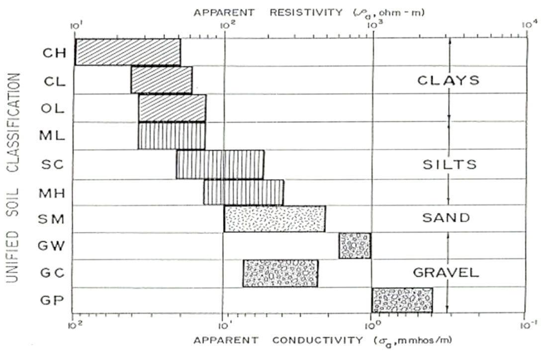
In-situ measurement of apparent resistivity of earth materials depends on several factors. The most important of these factors with respect to aggregates studies is clay content (Figure 2). In general, as the clay content of bulk materials increases, apparent resistivity decreases due to the increased electrical conductivity of the fine grains comprising clay.

Of secondary importance to this application are pore volume and pore fluid. The larger the pore volume contained within a sedimentary unit or rock matrix, the higher the apparent resistivity. This is mainly due to the extremely high resistivity of the air contained in the pore space that tends to increase the bulk resistivity. With respect to pore volume, resistivity is controlled largely by the constituent pore fluid. The less resistive the pore fluid (for example, brine or water rich in other total dissolved solids, TDS), the lower the apparent resistivity of the unit. More resistive pore fluids, such as hydrocarbons, tend to increase apparent resistivity.

Typically, electromagnetic (EM) and electrical methods are used to map apparent resistivity variations. EM instrumentation, including the widely used Geonics EM31, EM34-3 and EM38, exploit EM induction laws to obtain measurements of apparent conductivity.

Conventional electrical resistivity methods employ steel electrodes that are hammered into the ground. Direct current is injected through couplets of electrodes and resultant voltages are measured across separate electrode couplets. Systems in use today, such as the IRIS Syscal systems and the AGI Sting, use switch boxes to regulate measurement cycles over quartets of electrodes along linear arrays that can include a number of electrodes (commonly-used arrays include 48, 72 or 96 electrrodes). For obvious reasons, this approach tends to be time-consuming and labour intensive.

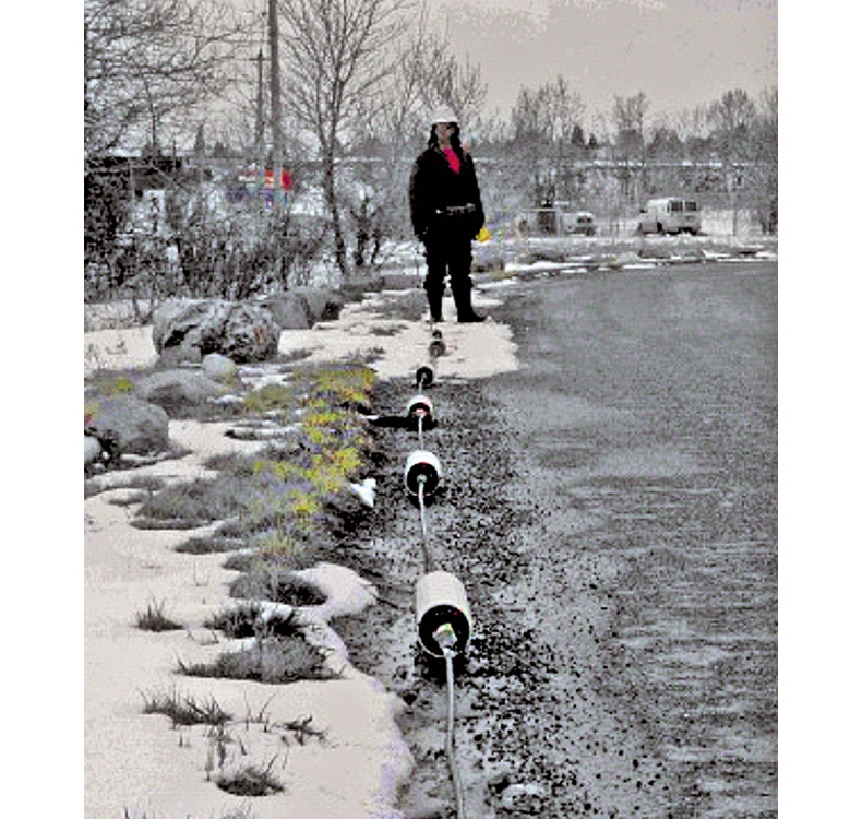
Manufactured by Geometrics Inc., the OhmMapper measures apparent resistivity by generating electrical current flow in the subsurface through capacitive coupling. Whereas conventional electrical resistivity systems directly inject current through metal electrodes driven into the ground, the OhmMapper applies a current to the ground using capacitive coupling between its transmitting electrical dipole and the subsurface. The OhmMapper system is illustrated in Figure 3 and consists of a transmitting antenna and associated dipole cabling, one or more receiving antenna(s) with associated dipole cabling, a fibre-optic isolator and a data-logging console.

As outlined in Morrissey (2010), the system functions by imparting current to the subsurface using the soils as the dielectric in a capacitive ‘circuit’ between the system and the subsurface. Current distribution within the subsurface varies as a function of the resistivity of the subsurface material and voltages generated by the current flow are sensed and recorded by the receiver dipoles. The receiver voltage depends on the transmitter voltage, the lengths of the dipoles, the separation of the transmitter and the receivers, and the resistivity of the subsurface. For any single measurement, receiver voltage is adjusted for the geometry of the transmitter-receiver arrangement and converted to an apparent resistivity. The dipole lengths and transmitter-receiver separations can be adjusted to assess apparent resistivities at different depths and with varying vertical resolution.

Whereas conventional electrical resistivity systems require the insertion of multiple electrodes into the ground, the capacitively-coupled OhmMapper is generally towed along the ground surface which affords it many practical advantages over conventional systems. System set-up and data acquisition are simplified and the data collection more rapid than with conventional resistivity systems. The OhmMapper is insensitive to contact resistance problems that plague conventional systems in the presence of gravels, bedrock and permafrost. Areas that have traditionally been off-limits to conventional systems, such as roads, asphalt walkways and frozen or well-compacted near-surface sediments, can be surveyed with the OhmMapper. As well, rough terrain that contributes to the high labour intensity of the conventional resistivity systems (e.g. heavy tree cover, thick snow, steep inclines) can be surveyed with greater ease as long as there are cleared survey lines.

Electromagnetic (EM) methods have also been traditionally applied to the problem of aggregate detection and delineation. These systems are useful for delineating lateral extent of lowconductivity regions associated with aggregates. However, these methods exhibit limited dynamic ranges, which can result in poor differentiation in high-resistivity/low-conductivity environments. Additionally, observed values of apparent conductivity are bulk values that reflect all of the material within the sphere of influence of the system. For example, using an EM31 in vertical dipole mode at ground surface will yield an effective depth of exploration of 6 metres. Measured apparent conductivities will thus have contributions from all of the material between the ground surface and 6 metres below surface, reducing its capacity to clearly resolve the depth extent of particular anomalies. The OhmMapper has a greater dynamic range (3 to 100 000 Ω@m for the OhmMapper compared with about 1 to 10 000 Ω@m) and significantly increased vertical resolution over EM methods. This is a distinct advantage when depth extent information is required for detailed resource analysis.

As with any geophysical method, the measurement of apparent resistivity is susceptible to limitations. As exploration depth is increased, vertical resolution decreases. A significant limitation of the OhmMapper system is its relative inability to penetrate electrically conductive media to great depth. The nominal depth of exploration of the system is 20 metres but this is crucially dependent on array geometry and subsurface conditions (i.e. material resistivity, temperature, pore volume and fluid as discussed above). In a situation where the target is beyond the depth capability of the OhmMapper, conventional (i.e. galvaniccoupling) electrical resistivity methods are required.

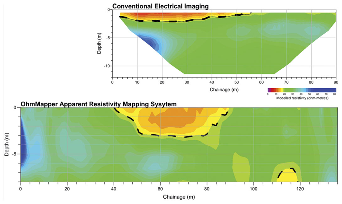
Direct comparison of OhmMapper data with conventional electrical resistivity imaging data collected in another part of Alberta (Figure 4) shows little variation between the two. Similar lateral and vertical extents of the primary anomaly (i.e. near the surface, 0 m) have been mapped by each method.

Results

The modeled apparent resistivity along survey line 13, an east-west transect in the northern portion of the survey area, is illustrated in Figure 5. Nine of the test pits advanced were located either along this line or immediately north of it (i.e. between 8 and 30 metres north of line 13). The geophysical and test pit data correlate well, which enhances the reliability of interpreted aggregate depths elsewhere in the survey area.

A contour interval of 118 Ω m was chosen as the lower limit of apparent resistivity with respect to the interpretation of the presence of coarse-grained aggregates. Modelled apparent resistivities greater than this cut-off are interpreted to be due to coarse-grained material while those under this limit are interpreted to be due to host material, for example lower-resistivity sand/silt/clay material.

All of the apparent resistivity crosssections generally indicate the presence of a shallow (less than 5.6 metres) resistor that has been interpreted to correspond to aggregates.

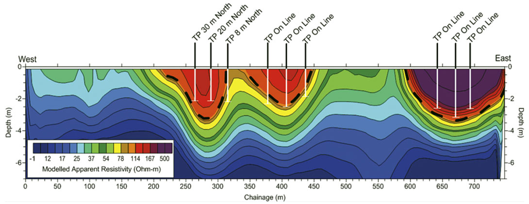
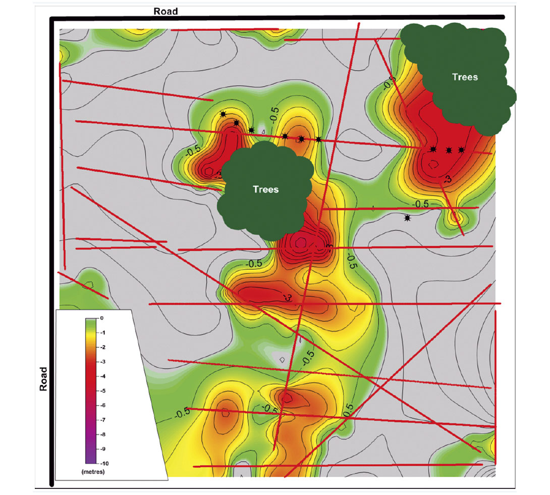
Figure 6 shows the lateral extent and maximum interpreted depth to the base of aggregates. The interpreted depths vary from 0 metres (reflecting the absence of coarse-grained material within the depth of exploration) to just over 5 metres in the centre of the survey area and are inclusive of the topsoil and silts that lie over the gravels (as noted in the test pits). Several small, high-resistivity anomalies appear along the northern, western and southeastern edges of the data that may indicate isolated regions of coarse-grained material.

A rudimentary estimate of aggregate volume can be derived from the isopach map of Figure 6 by treating the lateral variation in depth as the lateral extent of subsurface aggregates, i.e. determining the area bound by the 0-metre depth contour. The area can then be multiplied by average interpreted depth to base of aggregates, approximately 1.5 m, or maximum depth of interpreted aggregates, 5.6 m. These calculations yield approximately 323 985 m³ (about 518 376 tonnes gravel equivalent) and 1 209 544 m³ (about 1 935 270 tonnes gravel equivalent), respectively. These numbers are for illustration only and do not take into account such factors as the included fraction of non-gravel material, overlying topsoil, and elevation of ground surface. This is a first-level approximation that may be made from electromagnetic data, provided an estimate of depth extent is available through drilling or test pitting.

A more accurate volume estimate can be made by identifying an interpreted aggregate-bottom surface. Using the 3-D modeling software program Gemcom Surpac™, a volume estimate of 451 047 m³ has been derived, which is almost 40% greater than the rudimentary estimate using an average depth across the deposit. It is also 60% less than the volume overestimated from the maximum interpreted depth of aggregates. This more representative estimate can be used to develop an appropriate mine plan. Note that this estimate does not account for topography of the ground surface, which may affect total calculated volume of aggregates. It was also derived using the 0-metre depth contour as the lateral boundary of aggregate material without regard to the inclusion of non-coarse-grained material such as overlying topsoil or to lithologic variation within the ‘gravel’ unit, e.g. any sands or fine-grained materials that may be present. These factors introduce a degree of uncertainty into the volume estimate, and if known, should be applied (for example, decimate the estimated volume by a factor dependent on the ratio between sands and gravels).

Discussion and Conclusions

The results of the apparent resistivity survey show that the OhmMapper has successfully identified the presence of aggregate materials and has reasonably resolved their depth extent.

Note that, even though the test pitting shows the gravel unit to underlie between 0.33 and 0.85 metres of near-surface sediments, the OhmMapper does not have the resolution to distinguish the thin silts at surface given the acquisition parameters used. The data show (see Figure 5) resistive material extending from surface downward even though silts are relatively conductive.

The survey has highlighted some clear advantages that the OhmMapper has over more conventional electrical resistivity systems and electromagnetic methods. The most readily apparent of these is the time required to complete the survey. Twenty-two lines were acquired over two field days. It is estimated that 4 to 5 days would be required to acquire data along these lines with a conventional electrical resistivity system. In addition, the survey was conducted in November, a month when the ground is often frozen in central Alberta, suggesting that electrode insertion would be relatively labour-intensive.

Resolution of depth extent is a decided advantage over electromagnetic methods, which offer lateral resolution but poorly resolve vertical variations in subsurface conductivity. Figure 6 shows both lateral and vertical extents of the aggregates, an important consideration in determining the economic viability of the resource.

That is not to say that the OhmMapper is without limitation. In very conductive environments, the signal penetration of the OhmMapper can be so severely reduced as to render the system ineffective.

Since increased apparent resistivities tend to be associated with coarse-grained material, it is not possible to distinguish between sand and gravel. Therefore, it is always advisable to ground-truth the data through a programme of test-pitting or other intrusive investigation.

Factors such as permafrost and the presence of total dissolved solids can complicate interpretations by increasing the apparent resistivities of fine-grained sediments and decreasing the bulk resistivity of coarse-grained material, respectively. This understates the need for clear communications between client and geophysical service provider that include comprehensive descriptions of site conditions.

The OhmMapper has an effective depth of investigation on the order of 10 to 20 metres. It is, thus, not suited to cases where target depth is expected to exceed this range.

Collecting data over a systematic grid enables them to be presented as a pseudo-three-dimensional block model. This is advantageous because it facilitates lateral and vertical delineation of the aggregate resource, allows volume estimates of economically viable material to be made, and helps to select optimal locations for intrusive investigations.