In the challenging world of mapping thin stratigraphic targets, a geophysicist may choose to try a tactic for increasing resolution, particularly if it is simple, quick and has a known effect. The dipole filters described below, with either even or odd iterations (zero or 90 degree phase shift), can be used to "see" the details of a thinning layer through the fog of the lower frequency portion of a signal. In particular, a horizon with a doublet character may become split into separate events which can be "auto picked" more easily on a workstation. A catchy phrase to describe this method to landmen and engineers might be "first we catch the wave... then we ride the ripples".
The (1, -1) Dipole Filter
The dipole filter featured in this article (1, -1) consists of two time samples of equal amplitude with opposite signs. This filter has an approximately linear 6dB/octave slope, and a constant 90 degree phase shift (Anstey 1970). Successive convolutions re-apply the amplitude spectrum ramp and the 90 degree phase shift.
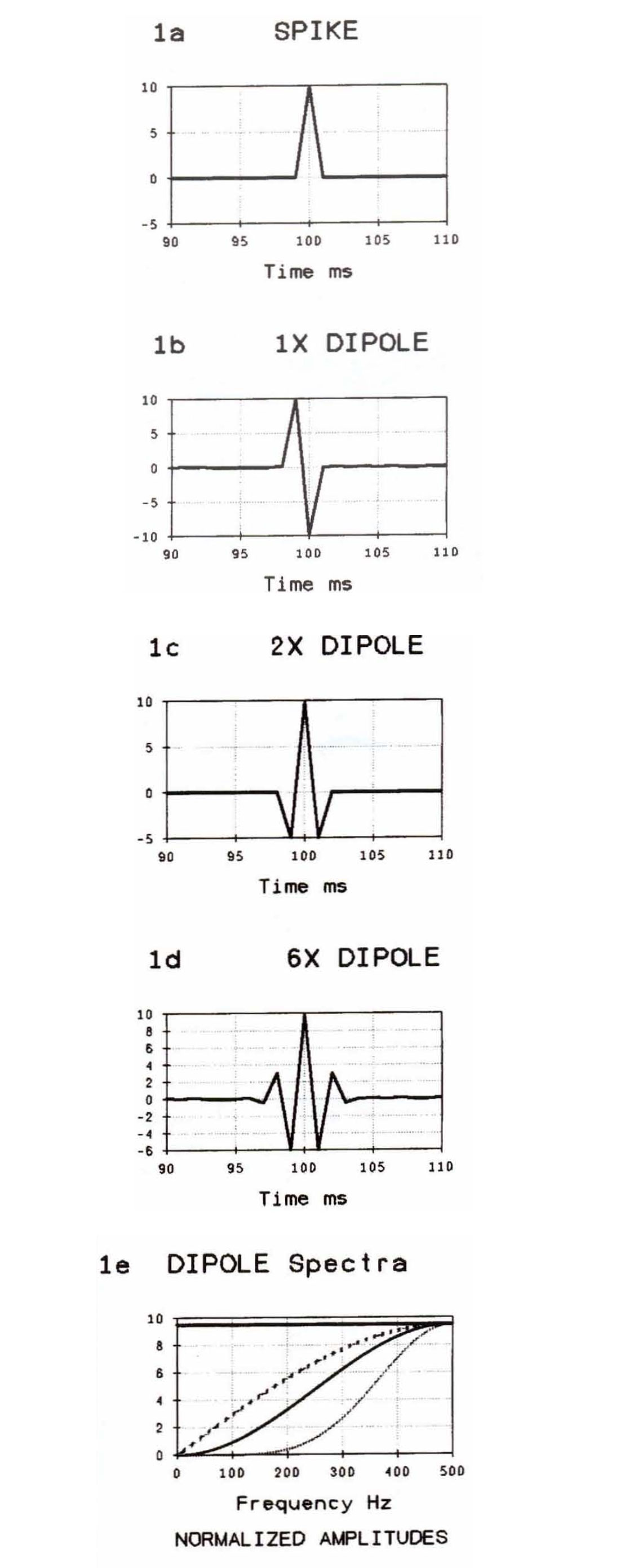
The dipole and even numbered cascades of two to six times with itself are shown in Figure 1. The cascaded filter becomes progressively longer and adds an extra lobe with each cascade. The amplitude spectrum is progressively enhanced at the high end and diminished at the low end.
Figure 1. Spike and amplitude spectra after successive convolutions with a) spike, b) dipole (1,-1), c) 2x cascaded dipole (-1,2,-1), d) 6x cascaded dipole (-1,6,-15,20,-15,6,-1) and e) the corresponding amplitude spectra. Sample rate 1 ms.
Derivatives
Both Anstey (1970) and Claerbout (1976) showed that this dipole is a digital approximation for differentiation of seismic data or wavelets. The subsequent cascaded convolution of the (1, -1) filter with itself, when convolved with the wavelet, approximates the second and higher order derivatives of the wavelet.
Resolution of Wavelets
Resolution of thin beds by a zero-phase wavelet is determined by the dominant frequency and the shape of its amplitude spectrum. The dominant period T, is the trough-to-trough time of the central side lobes. The corresponding frequency F=1/T is the dominant frequency. As a simple rule of thumb, the minimum seismic time separation for which the top and bottom of a layer can be clearly resolved as two separate time events is half the dominant period of the wavelet or T/2. (Widess, 1973; Kallweit and Wood, 1982). In this article the Raleigh limit R for temporal resolution is thus R=T/2.
Extending Resolution
The motivation for the use of these dipoles may be analogous to the motivation for the use of non-linear sweeps in Vibroseis recording, the use of higher low cut filters and higher natural frequency geophones, and several edge or fault detection strategies for image enhancement. The geophysicist is trying to extend the resolution of seismic layers.
What happens if we successively convolve or cascade this dipole with a seismic wavelet and with our seismic data? Will the amplification of the higher frequencies by the dipole enhance the resolution of stratigraphic events? Will this allow picking of isolated events that were previously merged in doublets or thin-layer tuning?
The illustrations that follow may generate discussion and experimentation with practical applications of these dipoles to assist in detailed interpretation.
Examples of Dipoles on Wavelets
The resolution effects of differentiation with cascaded dipoles are shown for a Ricker, an Ormsby, and a Butterworth filter in Figure 2 through Figure 4. The labels Tn and Rn will be used to refer to the period and resolution after n cascades of the dipole. Note that in each case the shape of the amplitude spectrum is multiplied by the ramp of each additional dipole. The low frequencies are attenuated and the higher frequencies are amplified. The dominant frequency increases as the dominant or central trough-to-trough period is reduced and additional lobes appear in the wavelet.
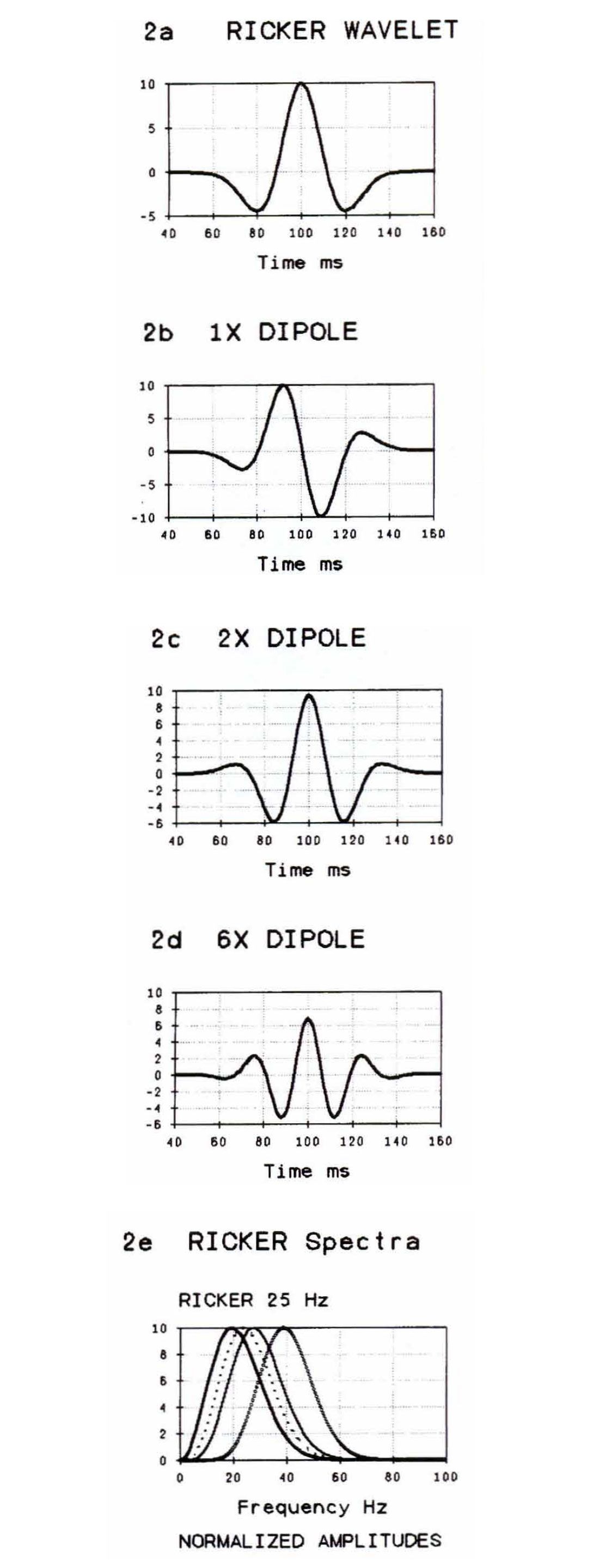
Figure 2. Ricker 25 Hz wavelet and amplitude spectra after successive convolutions with a) spike, b) dipole (1,-1), c) 2x cascaded dipole, d) 6x cascaded dipole and e) the corresponding amplitude spectra. Sample rate 1 ms.
Ricker Wavelet
The Ricker wavelet in Figure 2 has an initial dominant frequency of 25 Hz (corresponding to T0=40 ms, R0=20ms). The dominant frequency increases from 25 Hz to approximately 31 Hz (T2=32 ms, R2=16ms) and 43 Hz (T6=23 ms, R6=12ms) for the second (2x cascaded dipole) and sixth (6x cascaded dipole) derivatives, respectively. The bandwidth and time envelope stay approximately the same while extra side-lobes appear. The resolution is finer as the dominant frequency increases.
Ormsby Wavelet
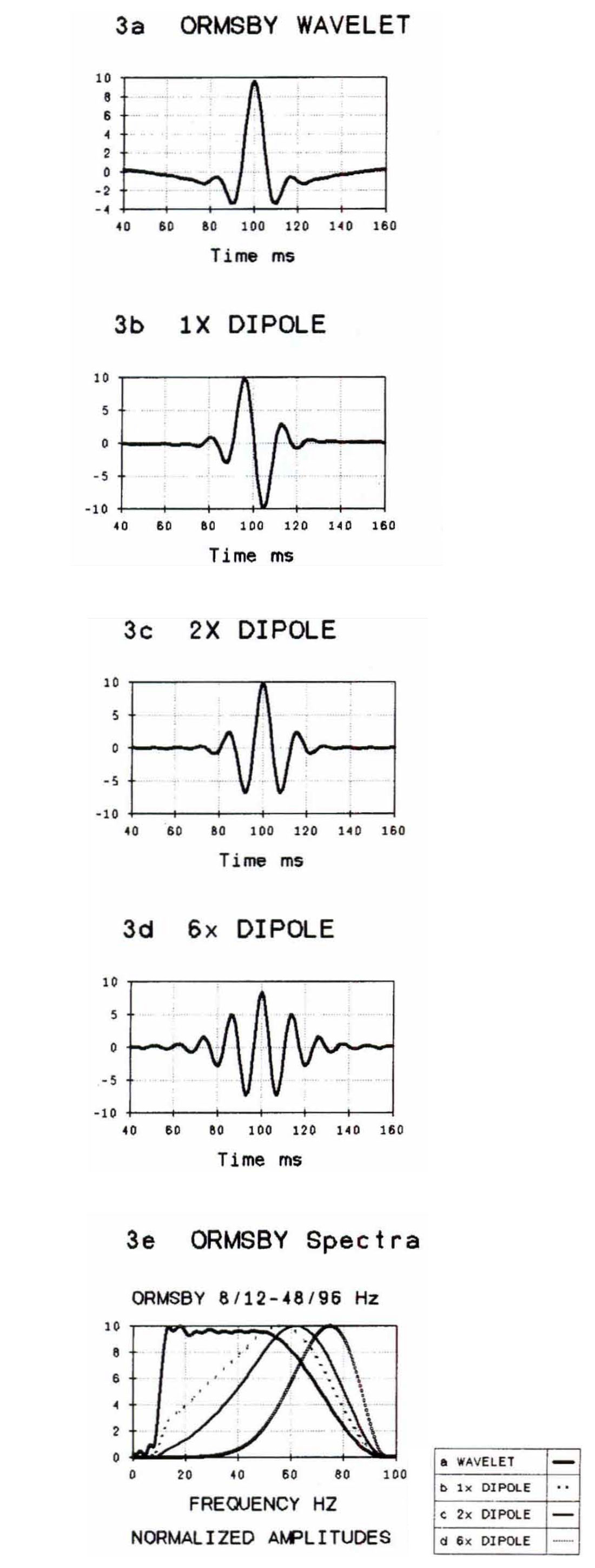
Figure 3 shows the dipole effect on an Ormsby type filter defined as 8/12-48/96 Hz.
Figure 3. Ormsby 8/12-48/72 Hz wavelet and amplitude spectra after successive convolutions with a) spike, b) (I,-I) dipole, c) 2x cascaded dipole, d) 6x cascaded dipole and e) the corresponding amplitude spectra. Sample rate 1 ms.
This filter has a bandwidth of 36 Hz equivalent to two octaves in width and a one octave high-end taper. The frequencies above 96 Hz are removed and cannot be recovered. The dominant frequency moves from 53 Hz (T0= 19ms, R0= 9ms) to 62 Hz (T2 = 16ms, R2=8ms) and 71 Hz (T6=14ms, R6=7ms) for the second and sixth derivatives, respectively. The initial side-lobes are exaggerated and the time envelope is lengthened. The ringy waveform is characteristic of the steep high-frequency cut-off of the resulting narrow bandwidth (see Appendix for further discussion).
Butterworth Wavelet
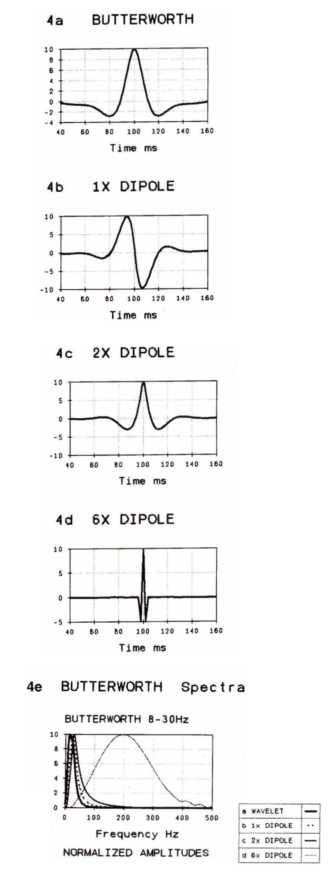
Figure 4 shows the dipole effect on a Butterworth wavelet (8 Hz@ 18 dB/octave-30 Hz@24 dB/octave). This filter was selected to illustrate the possibilities for enhancing an initially low frequency waveform provided the high frequencies, although weak, are present. The initial Butterworth filter has a low frequency side-lobe character with few visible side-lobes created after the series of cascaded dipoles. The dominant frequency moves from approximately 25 Hz (T0=40 ms, R0=20ms) to 40 Hz (T2=25 ms, R2= 12ms) and to 200 Hz (T6=5 ms, R6=2ms) for the second and sixth derivatives, respectively. While this improvement is beyond that expected in practice, this Butterworth wavelet will be used in 2-D stratigraphic examples in Figure 5 and Figure 6 to illustrate the potentially dramatic enhancement in resolution by cascaded dipoles.
Figure 4. Butterworth 8 Hz@/12 dB/octave-3D Hz@24 dB/octave wavelet and amplitude spectra after successive convolutions with a) a spike, b) (1,1) dipole, c) 2x cascaded dipole, d) 6x cascaded dipole and e) the corresponding amplitude spectra. Sample rate 1 ms.
Resolution and Interpretation Goals
The convolution of these short filters with the interpreter's zero-phase broadband data may raise the effective dominant frequency. Effectively the low frequency portions of the signal are reduced, and we can see the ripples on the waveform and refine our picking of events.
Resolution and a Wedge Model
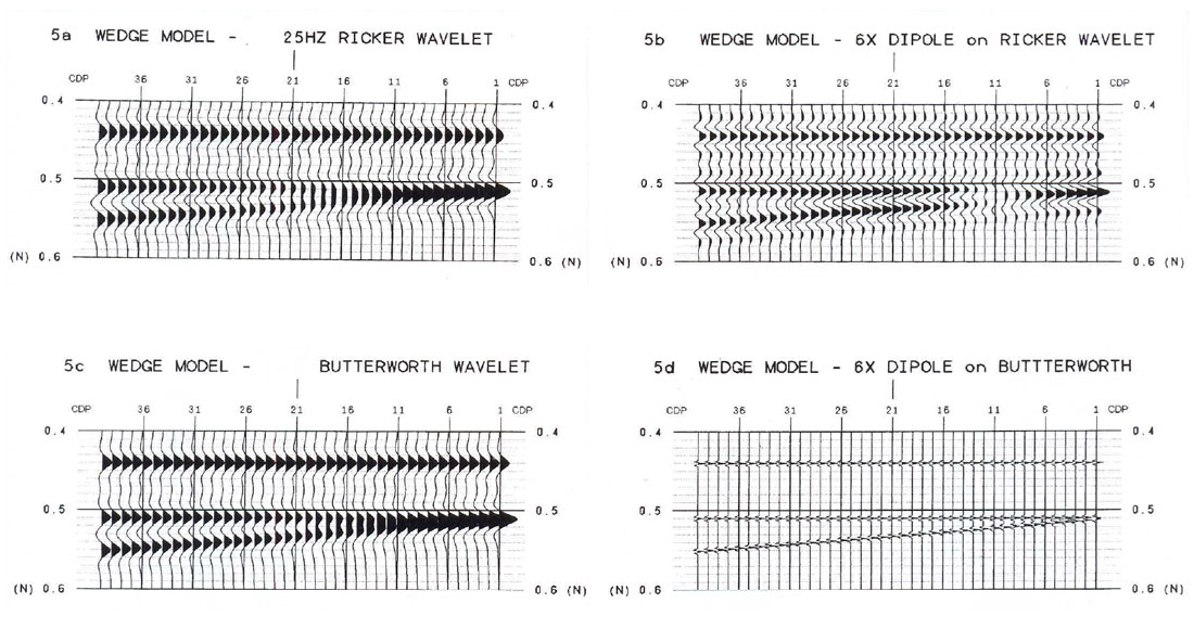
The effect of extending the limits of resolution are visually demonstrated in Figure 5 with a simple wedge model. The time separation between the equal amplitude positive spikes of this wedge increases by I ms/trace. Thus the trace number corresponds directly to the time separation in ms. Figure 5 shows the wedge model before and after six cascades of the dipole on the Ricker wavelet from Figure 2 and the Butterworth wavelet from Figure 4, respectively.
Figure 5. Wedge model with same polarity positive spikes with a) 25 Hz Ricker wavelet and b) after 6x cascaded dipole application. Figures 5c) and 5d) repeat 5a) and 5b) using the Butterworth wavelet 8 Hz@18dB/octave-3DHz@ 24 dB/octave. Model layer separation increases by 1ms per trace. Sample rate 1 ms.
Figure 5a and 5b show the before and after response of the wedge model with an initial 25 Hz Ricker wavelet corresponding to a dominant period T0 of 40 ms, for which the Raleigh temporal resolution is R0=T0/2=20ms. Figure 5a demonstrates this expectation with trace 20 being the first trace where the two events are separate. Figure 5b show the results after the application of the sixth derivative filter (i.e., the 6x cascaded dipole). A clear separation of two events can be seen on trace 12. This matches the expected resolution for the 6x dipole on this Ricker wavelet where T6=23ms giving R6=12ms.
Figures 5c and 5d show a more dramatic extension of the resolution limit for the same wedge model using the Butterworth wavelet from Figure 4a. The initial 8 Hz@18 dB/octave-30 Hz@24 dB/octave Butterworth wavelet has T0=40 ms with expected resolution R0=20 ms or less. Figure 5c shows the initial separation for the layers clearly identifiable at trace 16 (i.e., 16 ms resolution). After applying the 6x cascaded dipole we expect a resolution of R6=2-3 ms. The result in Figure 5d shows that the wedge is resolved at trace 2.
Resolution and a 2-D Synthetic Model
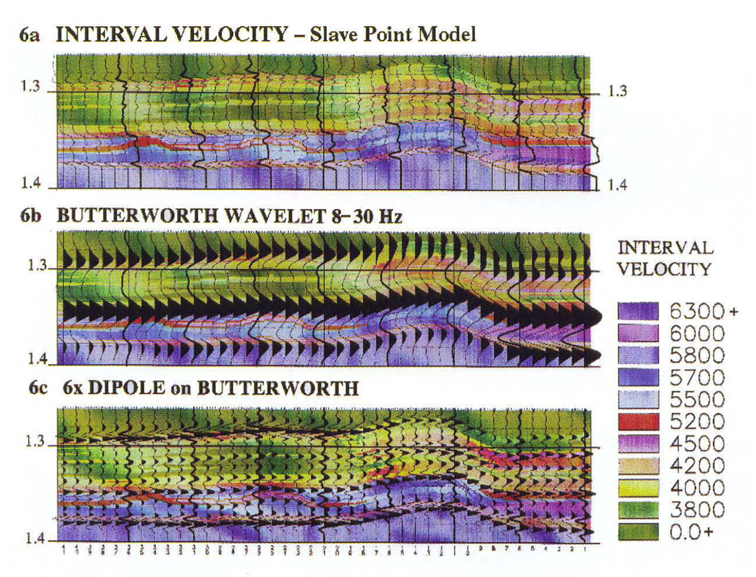
Figure 6 shows an example applicable to resolution issues in NW Alberta Slave Point patch reefs and illustrates the potential for these short filters to extend the resolution of thin layers below the initial apparent temporal resolution limit. Figure 6a shows the interval velocity model corresponding to a 20ms thick patch reef with basinal infill or porosity development. In Figure 6b the reflection coefficients are filtered with the rather low-frequency Butterworth filter from Figure 4. The effect of the sixth derivative cascaded dipole filter on this Butterworth synthetic is shown in Figure 6c.
Figure 6. 2-D stratigraphic Slave Point reef model in terms of a) model interval velocities, b) synthetic seismic section using the Butterworth wavelet discussed and c) after 6x cascaded dipole application.
Initially the character details of the reef are hidden as undulations in the shape of the waveform between the strong peaks on the synthetic. By taking the derivatives of Figure 6b to get Figure 6c we have separated the finer local events. The high-frequency "ripples" can be seen and can be more easily identified and interpreted.
Implications for Interpretation
These examples suggest that one might try the dipoles on seismic data until one gets the desired resolution or until the noise at higher frequencies becomes too strong to see coherent events. In practice, laterally incoherent noise may be reduced with FX deconvolution methods between multiple applications of the dipole.
On the seismic section the resulting improvement in resolution will move the onset of thin-bed tuning to a thinner bed thickness. Depending on the target thickness and the achieved wavelet resolution the interpreter may not need to switch between mapping strategies for time-based resolution to amplitude-based resolution of thin beds. Doublet events which could not be autopicked on a workstation may be split into separately pickable events.
Interpretation Strategy
The geophysicist attempts to retain a wide range of frequencies throughout the processing flow. The resulting final migrated section usually has a broadband, possibly flat spectrum of at least two octaves with good signal to noise ratio. The post-deconvolution interpretation wavelet is approximately zerophase, or made so by whatever method preferred by the geophysicist.
The selection of the final bandwidth and spectrum shape affect the limits and strategy used for resolution and interpretation of layers (see Appendix for further discussion). At any stage in detailed mapping, one might want to further refine the wavelet resolution. The dipole filters offer a method to enhance the effective higher frequencies and extend the limits of resolution of layer boundaries.
Future Work
We want to demonstrate the practical limitations of the dipole effects on several types of data and with different types of targets. We hope to show examples of the effects of these dipoles on the effective resolution of seismic data and the resulting refinement in the mapping of exploration or development targets.
About the Author(s)
Penny Colton is a geophysicist in the Interpretive Services group at Veritas Seismic Ltd. She received her B.Sc. in Physics from the University of Illinois in 1973. Following mineral exploration and graduate study at the University of Chicago she switched to seismic exploration with CGG in 1979. She was an applications geophysicist at Dome Petroleum (1981-1988) and subsequently in both exploration and development at Amoco Canada (1989-1992). She is an associate member of AAPG and a member of CSEG, CSPG, SEG, and APEGGA.
Atul Nautiyal is a consulting geophysicist with Lansdowne Exploration Ltd. Prior to consulting he was with Amoco Canada (1986-92), Numac Energy (1992-94) and Westward Energy (1994-96). Atul received a B.A.Sc. (engineering science-geophysics option) from the University of Toronto in 1984 and an M.Sc. (geophysics) from the University of British Columbia in 1987. He holds membership with CSEG, SEG and APEGGA. He is a former editor of the CSEG Recorder.
References
Anstey, N.A., 1970, Signal Characteristics and Instrument Specifications, in Evenden, B.S., Stone, D.R. and Anstey, N.A., Seismic Prospecting Instruments, Vol 1: Geopublication Associates, Geoexploration Monographs Series 1, No.3.
Berkhout, AJ., 1974, Related properties of minimum-phase and zero-phase time functions: Geophysical Prospecting, 22, 683-709.
Chung, Hai-Man and Lawton, D.C., 1995, Amplitude responses of thin beds: Sinusoidal approximation versus Ricker approximation; Geophysics, 60, 223-230.
_____ and _____ and , 1995, Frequency characteristics of seismic reflections from thin beds: Canadian Journal of Exploration Geophysics, 31, 32-37.
Claerbout, J.F., 1976, Fundamentals of geophysical data processing: McGraw-Hill Inc., 44-47.
De Voogd, N. and Den Rooijen, H., 1983, Thin layer response and spectral bandwidth: Geophysics, 48, 12-18.
Hunt, L., Gray, D. and Wallace, R., 1993, Using reflectivity to produce a superior deconvolution, 1992 CSEG meeting abstracts, 95-96.
Kallweit, R.S., and Wood, L.C., 1982, The limits of resolution of zero-phase wavelets: Geophysics, 47, 1035-1046.
Knapp, R.W., 1993, Energy distribution in wavelets and implications on resolving power: Geophysics, 58, 39-46.
_____, 1990, Vertical resolution of thick beds, thin beds, and thin-bed cyclothems: Geophysics, 55, 1183-1190.
_____ and de Voogd, N., 1980, The linear properties of thin layers, with an application to synthetic seismograms over coal seams: Geophysics, 45, 1254-1268.
O'Doherty, R.F., and Anstey, N.A., 1971, Reflections on Amplitudes: Geophysical Prospecting, 19, 430-458.
Ricker, N., 1953a, The form and laws of propagation of seismic wavelets: Geophysics, 18, 10-40.
_____, 1953b, Wavelet contraction, wavelet expansion and the control of seismic resolution: Geophysics, 18, 769-792.
Schoenberger, M., 1974, Resolution comparison of minimum-phase and zero-phase signals: Geophysics, 39, 826-833.
Szulyovszky, I., 1991, Resolution comparison of conventional and recursively inverted signals: Geophysics, 56, 242-244.
Walden, A.T. and Hosken, J.W.J., 1985, An investigation of the spectral properties of reflection coefficients: Geophysical Prospecting, 33 400-435.
Widess, M.B., 1982, Quantifying resolving power of seismic systems: Geophysics, 47,1160-1173.
_____, 1973, How thin is a thin bed?: Geophysics, 38, 1176-1180.
Ziolkowski, A. and Fokkema, J.T., 1986, Tutorial: The Progressive attenuation of high-frequency energy in seismic reflection data: Geophysical Prospecting, 34, 981-1001.
Appendices
Cascaded Dipoles
The filter samples for cascaded convolution of the dipole with itself can be calculated by polynomial multiplication of the Z-transform representation of the dipole:
(1 - z) * (1 - z) = 1 - 2z + z2
which corresponds to filter time samples of 1, -2, 1. This double convolution has an approximate 12 dB/octave slope and 180 degree phase. Within this article, we used the zero phase form of this filter with time samples -1, +2, -1 as the "2 times" or double cascaded dipole. The filter samples for the dipole and the "normal polarity" zero phase versions of cascaded convolutions of that filter are:
1 dipole:
1,
-1
2 times:
-1,
2,
-1
4 times:
1,
-4,
6,
-4,
1
6 times:
-1 ,
6,
-15,
20,
-15,
6,
-1
These cascaded dipoles are shorter than most deconvolution operators or other whitening techniques. While they can not replace deconvolution techniques, which correct the phase of the data while flattening the amplitude spectrum, and do not restore low frequencies, dipoles are a very powerful technique to amplify higher frequencies of zero-phase data.
Non-White Reflection Coefficient Series
O'Doherty and Anstey (1971) and Ziolkowski and Fokkema (1986) discussed the progressive attenuation of high frequencies caused by the transmission through thinner overlaying layers and the non-whiteness of reflection coefficient series. "Coloured" deconvolution techniques compensate for the observed character of log-based reflection coefficients. (Walden and Hosken, 1985 and Hunt, Gray and Wallace,1993). Often this compensation reduces the relative amplitude of the lower frequencies on a seismic section in a fashion similar to the dipole illustrated here.
Derivatives and Temporal Resolution
Ricker (1953a) reminded us that the relationship between first and successive derivatives is similar to the inherent relationship between signals detected on particle displacement, velocity, and acceleration detectors. Reflection coefficients are similar to a scaled derivative of the impedance series and one observes the expected relationship between the character and spectra of the impedance and reflection coefficient series. The related effect on resolution is discussed by Szulyovszky (1991)
The first and second derivatives of wavelets are the basis for several criteria used to define resolution for a given wavelet and the related onset of thin-bed tuning, usually illustrated by a wedge model (Widess, 1973; Kallweit and Wood, 1982). The Raleigh criterion for resolution is derived from the peaktrough timing (first derivative equal zero). The Ricker (1953b) criterion for resolution, using the detection of a flatspot in the combined waveform, is based on the time between the inflection points (second derivative equals zero).
Temporal Resolution and Bandwidth
Widess (1982) defined resolving power based on bandwidth alone for flat amplitude spectrums and defined an equivalent bandwidth for non box-spectrum wavelets. Knapp (1990) shows that with at least a couple of octaves in bandwidth, effective resolution of the time separation of thin beds is best improved by adding high frequencies. Knapp (1990) further concluded that "resolution can be improved by filtering away low frequencies if as a consequence of this filtering, higher frequencies are recovered".
When the band-range remains the same Koefoed (1981) showed the effect of spectrum shape on the dominant period and side lobes character. Similar effects are seen here when the maximum of a spectrum is skewed from flat toward the low, middle or high end of the bandwidth.
Dipoles and Frequency Domain Filters
The Ormsby type bandpass wavelet in Figure 3 demonstrates the caution side of Knapp's conclusion (1990) that filtering away low frequencies improves resolution, if as a consequence of this filter, higher frequencies are recovered. In this Ormsby example the application of the frequency domain trapezoidal filter prevented the subsequent recovery of higher frequencies by the dipole filters.
A similar ringy waveform character may result when the dipole is applied to Vibroseis or any data if frequency domain processing steps are restricted to a narrow frequency range. In that case the extension of resolution by the dipoles is limited to the reduction of the low frequencies without gaining additional higher frequencies.
Resolution and Amplitude Tuning
Widess (1973) in his classic, "How Thin is a Thin Bed?", and Kallweit and Wood (1982) have shown that for given wavelets (Ricker and boxcar-type spectra) there is a certain layer thickness beyond which amplitude tuning rather than time separation must be used to resolve the layer thickness. The amplitude tuning curves must be modeled for the given wavelet and the specific type of wedge model. The examples in Kal1weit and Wood (1982) summarize the effect of thin bed tuning for the both the case of same polarity (Ricker, 1953b) and of opposite polarity (Widess,1973) equal-amplitude reflections from the top and bottom of a thin wedge. Chung and Lawton (1995) expanded the resolution analysis for cases of unequal amplitude reflections.
For thin-bed targets, De Voogd and den Rooijen (1983) suggested changing the dominant frequency of the wavelet to put the target layer time thickness either below or above the transition zone between clear temporal resolution and the amplitude based resolution of thin-beds.
In a detailed analysis any two closely spaced events do themselves act as another two point dipole filter, and their relative polarity and amplitude do effect the exact resolution limits and the selection of an appropriate identification strategy. The understanding of the desired resolution, obtainable with a given dominant frequency and spectrum shape, and the limitations of the signal to noise ratio of the data can guide decisions about when and how many times to try dipole filters to enhance resolution.
Recommendations
Although we are by-passing details here, in general we recommend calibrating the interpretation strategy after extending the resolution of targeted layers. Use similar wavelets and amplitude spectra shapes to compare the character and resolution of events on 2D synthetic models with the final seismic data.
Join the Conversation
Interested in starting, or contributing to a conversation about an article or issue of the RECORDER? Join our CSEG LinkedIn Group.
A large volume of data is being converted to make this online archive. If you notice any problems with an article (examples: incorrect or missing figures, issue with rendering of formulas etc.) please let us know by emailing:
admin@csegrecorder.com


Join the Conversation
Interested in starting, or contributing to a conversation about an article or issue of the RECORDER? Join our CSEG LinkedIn Group.
Share This Article