Calibrated AVO and LMR analysis using a new DHI flat-spot AVO class 6 fluid contact to mitigate reservoir risk at Stonehouse, offshore Nova Scotia

Abstract

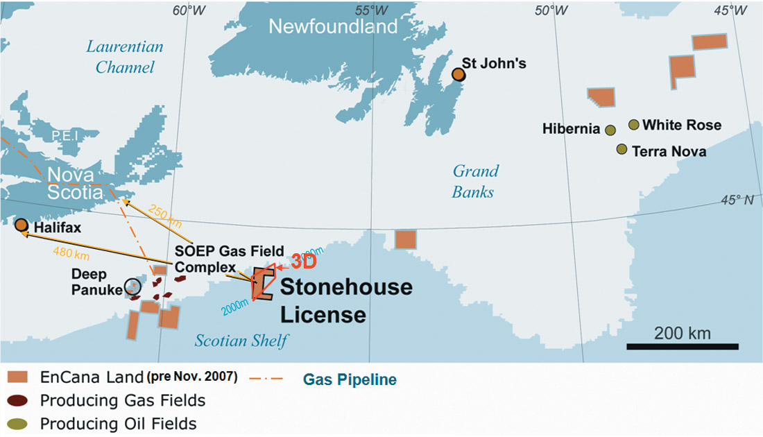
This article describes the Amplitude Variation with Offset ( AVO) and Lambda-Mu-Rho (LMR) analysis that followed the Pre-stack Depth Migration (PSDM) of a 2,000 km² 3D covering the shallower, prospective part of the relinquished deep water Stonehouse license offshore Nova Scotia (Figure 1).

AVO analysis and LMR attribute inversion are routinely used to reduce reservoir risk in offshore exploration drilling. However, AVO can only detect relative anomalies due to high porosity hydrocarbon filled reservoirs, whereas log-calibrated LMR inversion can provide a quantitative extraction of rock properties to discriminate lithology, porosity and fluids given reasonable data quality and amplitude preserved processing. The motivation for AVO/LMR analysis on the Stonehouse 3D stems from the failure of the majority of Scotian slope wells drilled to intersect economic reservoir sands.

In order to be able to discriminate high porosity sands from sub-economic low porosity sands, various AVO/ LMR responses to fluid and porosity variations were predicted through Biot-Gassmann Fluid Replacement Modelling (FRM) as well as porosity substitution and thickening of thin, low porosity target gas sands from the nearby Tantallon (M-41) well. As the M-41 well has no shear dipole data so log data from the Annapolis (G-24) gas discovery well provided background P-wave to shear-wave mudrock velocity relationships. In addition, the G-24 logs afforded a critical verification that the higher porosity substitution (from 9% to 18%) of the gas charged sand zone in M-41 matched the stratigraphically equivalent 18% porosity gas sands encountered in G-24 from both a petrophysical and AVO/LMR perspective.

Synthetic AVO models of gathers and wedge thicknesses ranging from zero to 50m were created for the 9% porosity insitu gas saturated sands and the 18% porosity substituted case, using various gas/brine saturations. These wedge models and the FRM predicted that high porosity substituted gas sands produce very bright AVO class 3 or 4 responses at thicknesses > 10m. By contrast, low porosity gas or brine sands had near zero contrast to background shales with dim AVO class 2 gather and stack responses, while the 18% porosity brine sands showed only marginal AVO class 1 contrast.

Beyond standard LMR (λμρ) cross-plotting that successfully isolated gas sand clusters in the M-41 log data, an improved separation of high porosity sands was further achieved using a λρ–μρ? difference vs. acoustic P-impedance (Ip) template. When applied to the calibrated AVO/LMR attributes inverted from the 3D, the λρ–μρ? difference vs. Ip cross-plot analysis permitted a more discriminating and believable isolation of prospective gas sands than standard LMR.

Following the modified Rutherford and Williams scheme of AVO classes 1 to 5 (Young et al 2003) and at the risk of over classification, a new AVO class 6 fluid-only GWC is defined in terms of P-wave (Rp) vs. shear-wave (Rs) reflectivity as opposed to Intercept (I) and Gradient (G). The theoretical gradient modelling of this class 6 is used to validate a structural flat-spot identified on the migrated stack by mapping its structural conformance to a salt dome flank. This DHI fluid contact control point was critical in the cross-plot data template masking and polygon projection onto the 3D volume. Along with further attribute analysis, the DHI template confirmed that troughpeak reflectors up-dip from the flatspot occupied the same cross-plot region as the 18% porosity gas sand model and were generally sparsely (hence discriminately) populated throughout the 3D.

Sand body depth volumes projected from cross-plot polygons using LMR and AVO intercept-gradient reconnaissance analysis were combined with independent, seismic-stratigraphic interpretation in Landmark’s GeoProbe enabling improved constraints on resource estimates. The detailed AVO analysis also permitted a more confident assessment of the reservoir risk at the objective horizons.

Introduction: 3D reprocessing, interpretation and mapping

The Stonehouse 3D covers a stratigraphically complex structural prospect located on the Scotian slope. The 3D was originally processed through pre-stack time migration (PSTM) following the application of the best available 2D Surface Related Multiple Elimination (SRME) method. However, it was evident that the data were still contaminated by residual water-bottom focused multiple diffraction energy and that PSTM was unable to correctly compensate for travel time “statics” caused by the extremely rugose sea floor.

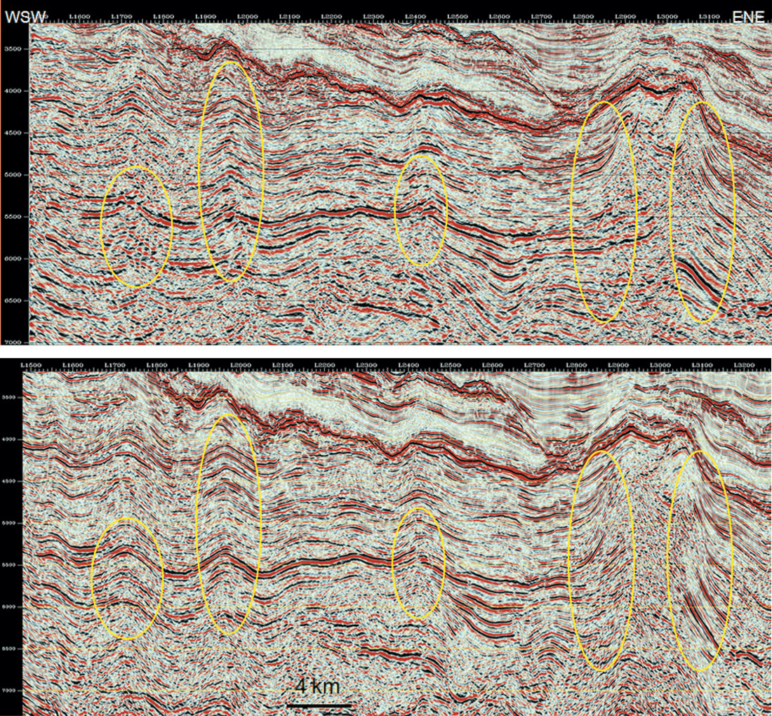
Consequently, the 3D was reprocessed to incorporate new and improved 3D SRME demultiple methods as well as pre-stack depth migration (PSDM). The velocity model building was undertaken using a hybrid, layer- based, gridded-cell tomographic scheme and the data were depth migrated to 12 km using a Kirchhoff algorithm. Figure 2a and 2b, show a comparison of the original PSTM processing and the 2006 PSDM processing (in time) on a strike line from the 3D. Note how the depth migrated section has corrected the miss-focusing of faults and folds due to the WB “statics” mentioned above, that are evident on the PSTM section (Mojesky et al 2007).

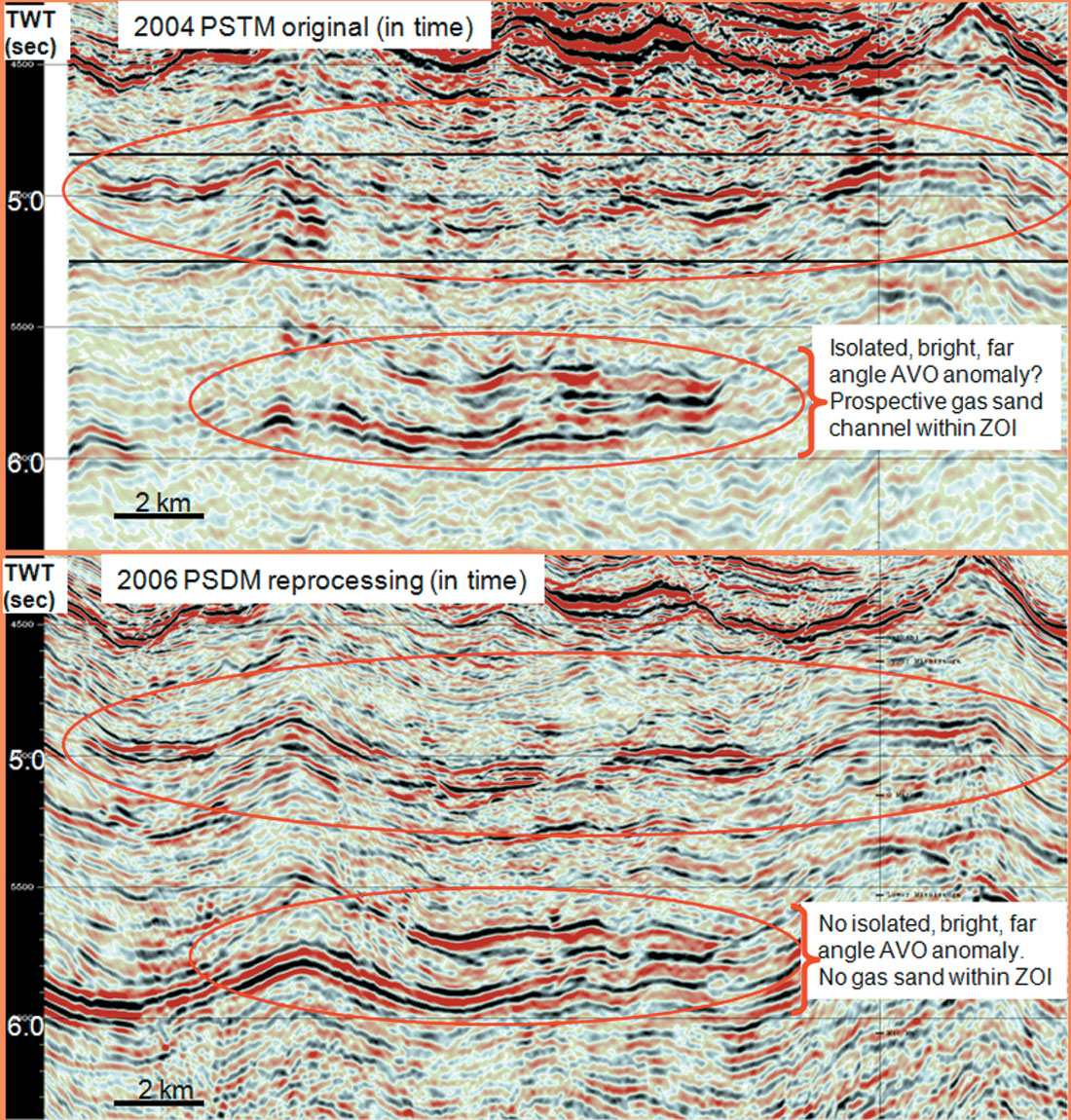
Of greater importance however, is the more moderate approach to multiple and noise attenuation that resulted in this new 3D volume having significantly broader bandwidth amplitude preservation that was now amenable to critical AVO/LMR analysis. This can be seen in figure 3 where an apparently well isolated far angle (30°- 40°) AVO amplitude anomaly seen in the original PSTM processing, is no longer evident on the PSDM reprocessing.

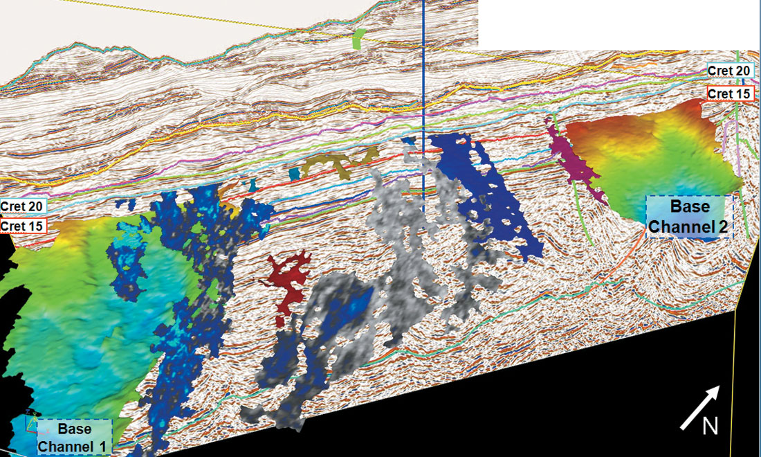
Interpretation of the new data clearly identified submarine canyons/channels throughout the target Cretaceous section that could have transported coarse sediment to the Stonehouse prospect. Figure 4 shows an arbitrary line from the 3D volume with interpreted channels and ‘geobodies’ in the primary objective interval. However none of these ‘geobodies’ necessarily contain gas charged reservoir with sufficiently high porosity to warrant exploration drilling. Detailed AVO analysis that follows, is the only method that has the chance to confirm if any of these bodies are in fact potential exploration targets and that their combined volume exceeds the economic hurdle for field development.

AVO and LMR analysis: modelling, fluid and porosity substitution

AVO/LMR analysis formed a crucial element of the technical evaluation as, arguably, high porosity reservoir presence is the only major risk to mitigate at Stonehouse. AVO extraction of P-wave and shear-wave reflectivity (Gidlow et al 1992, Fatti et al 1994) enables detection of relative anomalies due to hydrocarbon-filled reservoirs while LMR inversion (Goodway 2001), especially when underpinned by log-based calibration, allows for better discrimination of rock properties.

A careful petrophysical analysis of the Tantallon M-41 well located along strike some 50 km south-west of Stonehouse identified two, thin, low porosity gas-charged sands in the Cretaceous lower Missisauga 15-20 interval that are shown in figure 5. The thickest of these sands at 5210m MD is approximately 10m with 9% porosity and 60% gas saturation. This sand was chosen for the fluid and porosity substitution as well as for modelling the AVO gather and wedge thickening response, being the most representative target zone analogue that might be expected at Stonehouse.

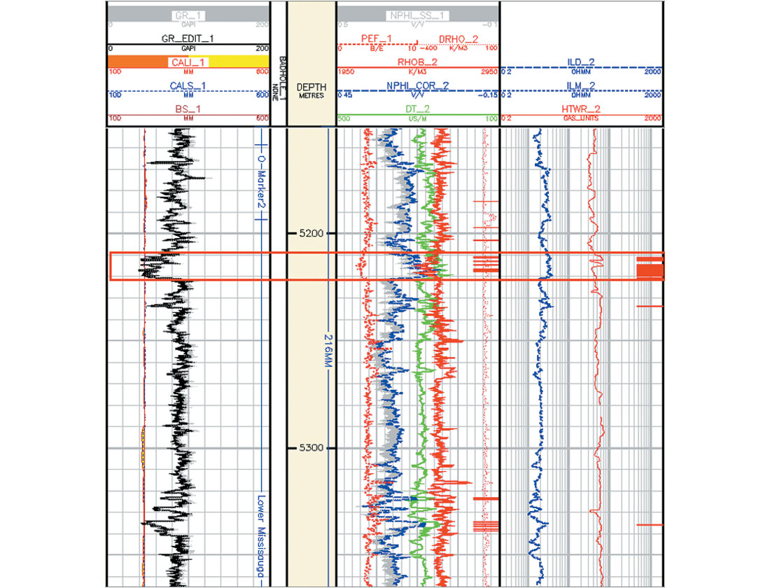
Figure 6 shows a busy composite cross-plot display of LambdaRho vs. MuRho, that does however capture all the results from the FRM and porosity substitution run on both the Tantallon M-41 target log, along with the known Annapolis G-24 gas sand and shale background, as well as its subsequent oil/wet sand fluid substitution. The correct Vp/Vs background mudrock relation for the M-41 substitution was established from dipole shear logs measured over the equivalent stratigraphic and depth range in G-24.

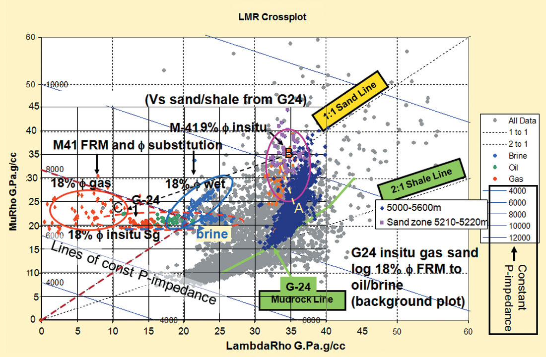
The cross-plot clearly demonstrates that the substitution of 18% porosity for the gas sand with in-situ (60%) gas saturation in M- 41 plots in the same region with low λρ and intermediate μρ as the known gas sand at the Annapolis G-24 discovery (area marked C). The fluid λρ only FRM shift to the right (horizontal blue arrow within dashed red oval) for the G-24 log moves the red gas points (5-16 G.Pa.g/cc) through slightly higher green oil saturated λρ values (16-20 G.Pa.g/cc) to fully saturated brine shown in blue (20-27 G.Pa.g/cc).

Validation of the FRM and porosity substitution for the M-41 zone of interest can be seen by closing the “LMR loop” on the cross-plot in figure 6. Starting from the shale background at point A established from the G-24 Vp/Vs green mudrock line and moving up the yellow diagonal “lithology” arrow from A (shale line) to B (sand line) separates the low, 9% porosity in-situ gas sand from shale. The porosity substitution from in-situ 9% to 18% can be followed along the black diagonal arrow from B to C, where the modelled M-41 red gas sand points match the actual G-24 gas sand points for economically flowable gas sand reservoir, as mentioned above. Finally, the λρ only gas to wet fluid shift for the M-41 log data following the horizontal blue arrow, represents a gas water contact in reflectivity contrast that is defined as a new AVO class 6 DHI later in the article.

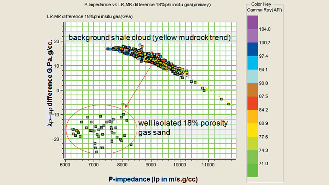
Despite the success of the standard λρ vs. μρ cross-plot approach in isolating the direction shifts for lithology, porosity and fluids, a better DHI and high porosity reservoir discrimination can be achieved by cross-plotting λρ−μρ difference versus P-impedance (Ip) as shown by the brown, dashed, triangular wedge on the left side of figure 6. Figure 7 shows how well this λρ−μρ versus Ip cross-plot separates the 18% substituted M- 41 gas sand zone from background shale. From this cross-plot, cutoff values below 8000 m/s.g/cc for Ip and negative λρ−μρ difference were chosen as quantitative limits to be used in the 3D data analysis discussed below. Note that the actual measured values for the 18% porosity gas sand in the G-24 well also fall within these cutoffs.

AVO gather and wedge thickness modelling

Figure 8 shows the synthetic gathers that were produced following fluid substitution of 100% wet and 90% gas for the in-situ, 9% porosity, 60% gas-saturated sand zone in M-41. The porosity was then increased to 18% while maintaining the same sand thickness and fluid substitution was rerun for 100% wet and 60% gas saturation. The resulting Vp/Vs logs show a clear drop even for a 60% gas charged 18% porosity sand, confirmed by using log control from the equivalent stratigraphic zone in the Annapolis G-24 well.

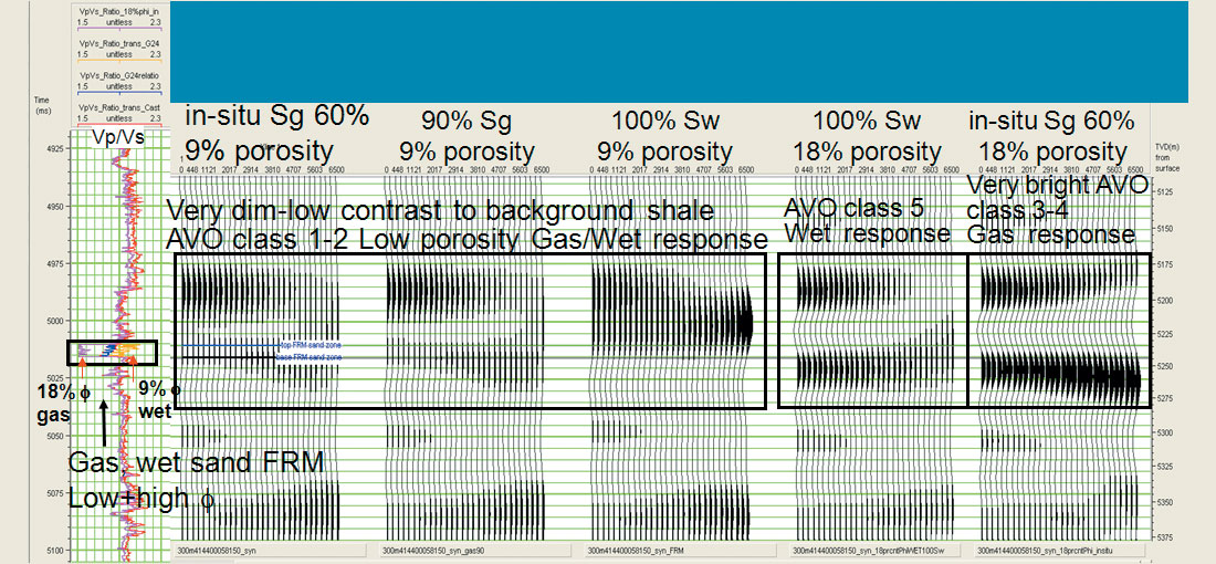
Synthetic gather modelling results of the FRM substitution show that for the 9% porosity sand, the AVO response would be a muted and weak AVO class 1-2, with only a subtle change due to 90% gas substitution for the 100% wet case. In fact, the 90% gas substitution has almost no effect for the uneconomic gas sand case; a good prediction given that the aim is not to repeat the drilling result from Tantallon. By contrast, the 10m, 18% porosity substituted sand with in-situ 60% gas saturation produced a very bright AVO class 3-4 response ( increasing to flat gradient), that was distinguishable from the AVO class 5 (decreasing gradient) for the 18% porosity wet case (see Figure 8).

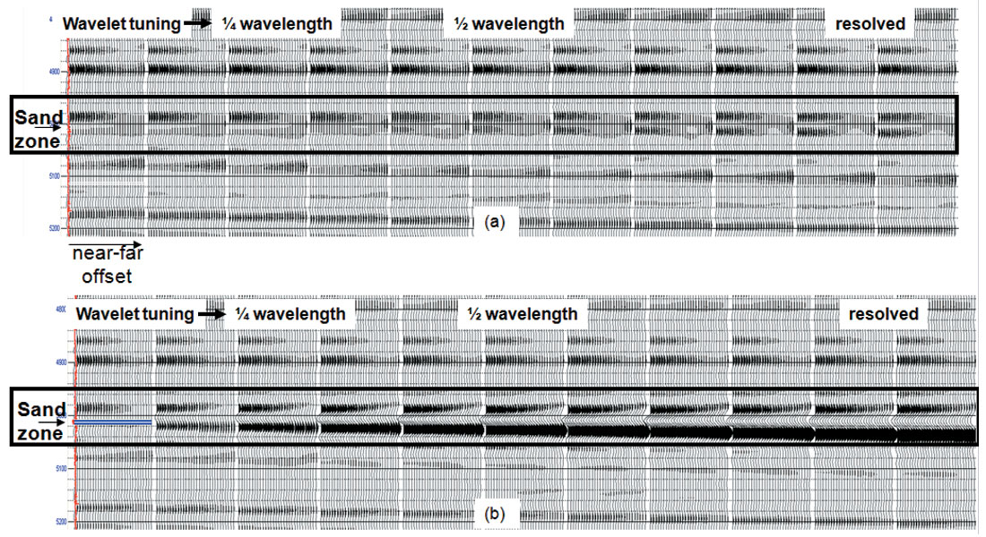
A wedge model of AVO synthetic gathers was run to compare the 9% porosity and 18% porosity in-situ gas case, in 5m thickness increments, varying from zero to 50m (left to right panels in Figure 9). The results show that for the 9% porosity gas case, only negligible changes to the dim AVO response are seen even at fully-resolved thicknesses. The 18% porosity gas sand however, is quite bright at the tuned 10m in-situ thickness and continues to brighten with increasing thickness.

These encouraging results from the modelling and fluid/porosity substitution feasibility work provided the impetus to proceed with the AVO/LMR inversion.

Flat-spot fluid-only contact identification: DHI AVO type 6 classification and modelling

Many claims have been made for post-stack interpretation of structurally flat, cross-cutting reflections termed “flat-spots” as fluid contacts i.e. the ultimate DHI. However, the AVO basis for these claims is either rarely examined or never published (excepting Dutta and Ode’ 1983). Furthermore the theoretical AVO classification of these “flat-spots” as fluid-only contacts that have been published, are flawed as shown in figure 10 (Isaacson and Neff 1999). To the author’s knowledge, seismic pre-stack analysis of the AVO signature for a post-stack flat-spot representing a true fluid contact is generally not conducted but warrants a deeper investigation given the unequivocal DHI potential in establishing a true AVO fluid contact as opposed to just a post-stack structural flat-spot.

The introduction here of an additional AVO class 6 emphasizes the importance in recognizing this classification as a distinct DHI and not just part of the base of the standard top-base (conforming and nonconforming) sand AVO classes 1 to 5 and -1 to -5 respectively, as described by Young and LoPiccolo in their 2003 TLE article. Furthermore a better understanding and isolation of the true AVO class due to a pure hydrocarbon effect, is fundamental in understanding 4D changes due to production and injection of fluids.

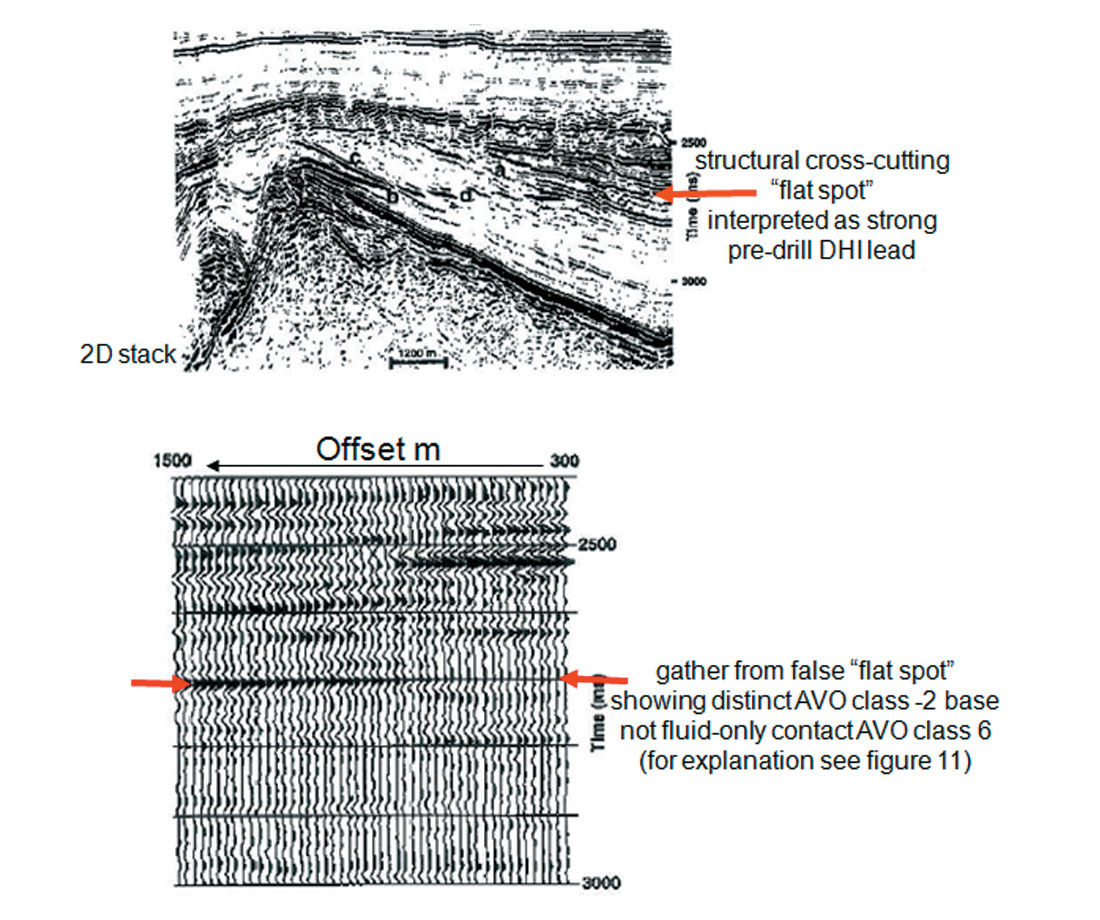
Figure 10 shows a 2D stack and gather data reproduced from the pre-drill Isaacson and Neff AVO publication from offshore Greenland. The stack section has a fairly convincing cross-cutting event at 2700ms (publication figure 7, marked b-d) with a representative gather of the flat-spot showing a distinct AVO class -2 base with zero intercept and a strong increasing peak gradient (lower panel; publication figure 13). Unfortunately the well that was located on this flat-spot and AVO prediction encountered a cross-cutting diagentic layer of recrystallized quartz within a thick, dipping shale sequence. The structural flat-spot interpretation was correct as the diagnetic recrystallization does in fact form along a horizontal cross-cutting plane, but the AVO prediction of a fluid contact as an AVO class -2 base was wrong. An explanation of this erroneous AVO class -2 base interpretation and the correct AVO type 6 prediction for a fluid-only contact, is shown in figures 11 and 12. The cross-plot in figure 11a, shows a theoretical Rp (x-axis) vs. Rs (y-axis) reflectivity “circle” plot with the standard top reservoir AVO classes 1 to 5 and the new AVO class 6 (red segment) for a fluid-only hydrocarbon/water contact. This new class 6 plots on the right side of both the top/base sand 1:1 line separation and the zero gradient 1:2 line (dashed), as well as on the positive side of the Rp xaxis. This location in the cross-plot can be simply understood from the fact that a pure fluid change only affects incompressibility Lambda (λ) and not the rigidity Mu (μ) within the P-wave modulus (λ+2μ) or P-impedance contrast, hence the Rp reflectivity. The Rp sign must be positive due to an increase in Lambda, but only slightly so, depending on the incompressibility contrast between the fluids involved in the flat-spot contact and magnitude of reservoir porosity.

For Rs shear-wave reflectivity on the other hand, a class 6 fluid-only contact will plot near zero on the y-axis, as a fluid change alone produces little or no change in shear impedance contrast, as Rs is mostly affected by its single rigidity modulus Mu. A slight modification however, due to a change in the fluid density across a flat-spot contact, means that a perfect zero Rs response is not possible thus complicating the class 6 location in the cross-plot. In fact, the result of a density increase in going from say gas to brine at the flat-spot contact would place the red GWC oval in figure 11a, slightly in positive Rs space above zero on the y-axis. With this understanding, the interpretation of an AVO class -2 base response (purple oval in figure 11a) shown by Isaacson and Neff in figure 10, as representing a pure fluid flatspot contact, is now evidently incorrect being located on the Rs y-axis instead of the Rp x-axis of the correct class 6 red oval in figure 11a. The class -2 base plots in the zero Rp range i.e. a total lack of near offset amplitude as seen in figure 10, implying an opposed change in both Lambda and Mu as the P-wave modulus λ + 2μ must remain constant for no P-impedance contrast. Furthermore, this zero Rp reflectivity also indicates a lack of density contrast that cannot represent a fluid contact as compressible fluids such as gas and brine exhibit strong differences in density.

In conclusion, the AVO class -2 base response shown by Isaacson and Neff in figure 10 must be due to a lithology contrast and not a fluid contact despite its flat-spot appearance in the stack section. This understanding might have avoided the subsequent drilling that encountered a lithologic change from a diagenetic quartz flat-spot within a thick shale and not the hoped for hydrocarbon-water contact.

The various AVO class curves shown schematically in figure 11b, that correspond to the AVO classes shown in the cross-plot in figure 11a, can be established from the two term linearized Aki and Richards angle dependent AVO reflectivity equation (1) as developed by Fatti, Smith and Gidlow.

Intercept and gradient responses predicted from this equation would be very different for AVO class -2 base sand reflections compared to class 6 for a pure fluid contact such as gas over water.

This can be seen by comparing the following equations (2) and (3):

The class 6 AVO gather response has a positive Rp intercept with a slightly increasing positive gradient due to the change in fluid incompressibility Lambda and density, while the class -2 base sand response has a zero intercept and a stronger positive gradient. These differences in gradient amplitude between class 6 and class -2 can be deduced from the cross-plot in figure 11a. The red GWC fluid class 6 is close to the zero gradient line due to zero Rs reflectivity, unlike the red class -2 base (purple oval) that has a strong gradient due to its large Rs reflectivity (also seen in equations (2) and (3) above).

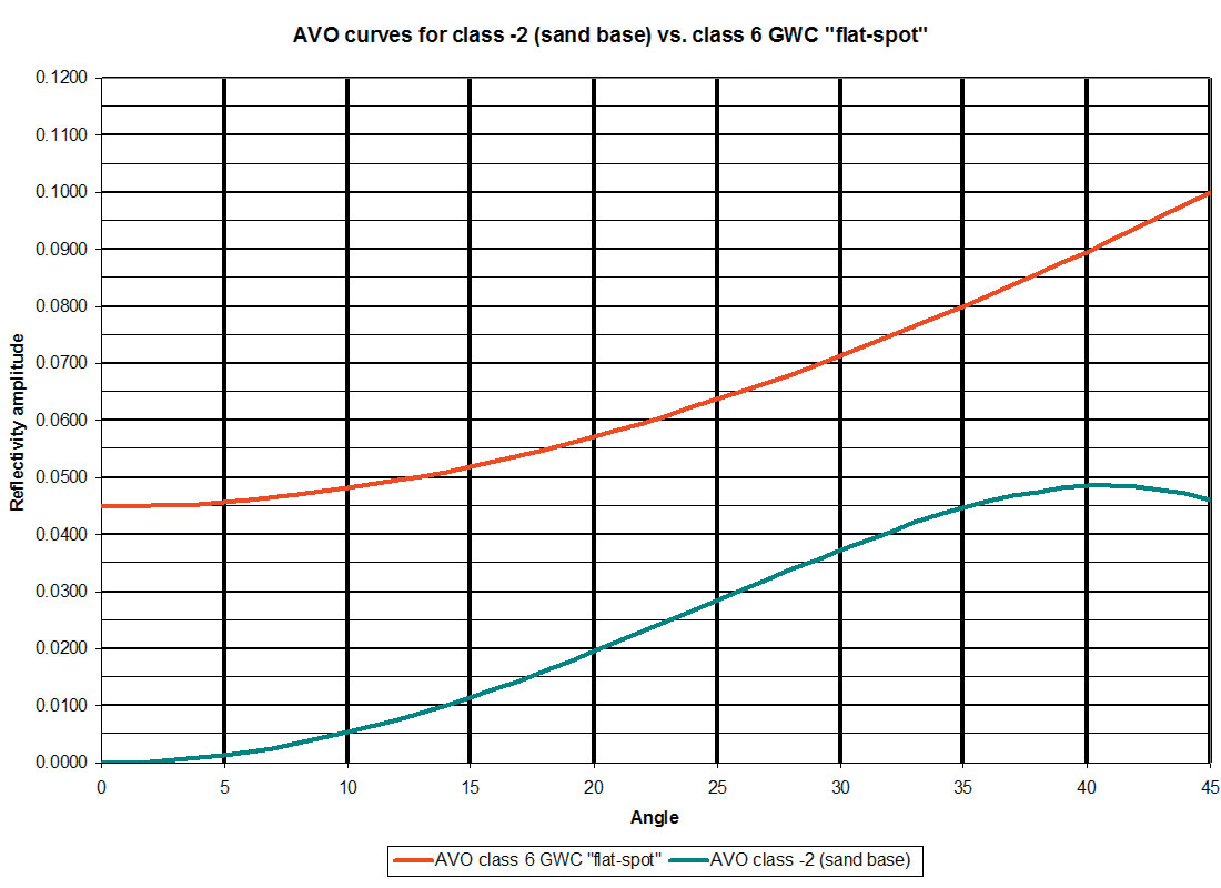
Actual theoretical comparisons of AVO curve responses, shown in figure 12, are based on the fluid and porosity substituted M-41 log as well as the Isaacson and Neff paper. Up to an incident angle of 30º the green class -2 AVO gradient is nearly 1? times that of the red GWC AVO class 6 response. In addition to their magnitude difference, the gradient curvature shapes for the AVO class -2 compared to class 6 fluid-contact, are distinct. As the class 6 is a function of tan2θ (equation 3) it has no inflection beyond 30º incident angle, while the class -2 has a clear inflection being a function of sin2θ (equation 2).

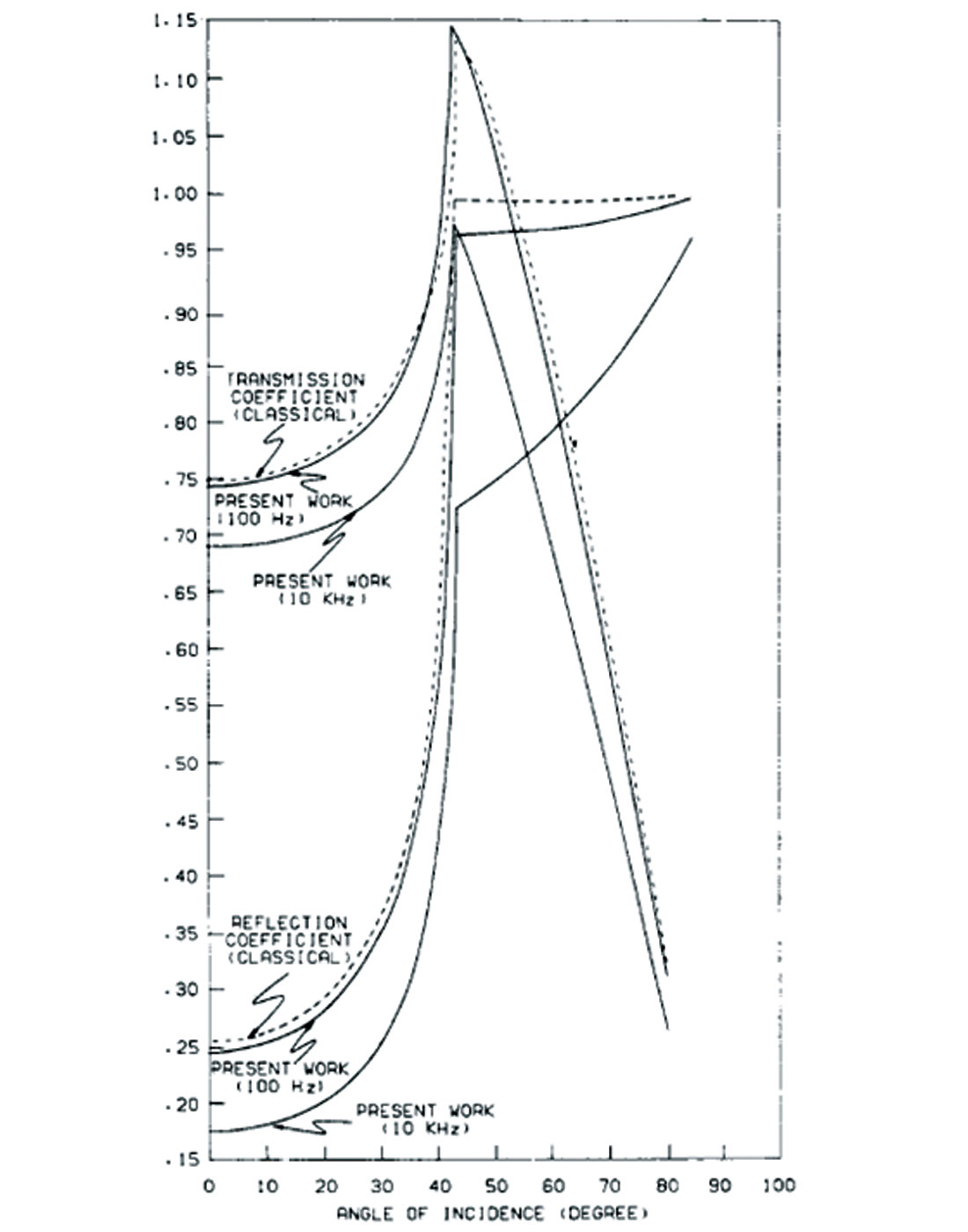
Confirmation of a class 6 AVO response as having a small Rp intercept and slight positive gradient is shown by the lower set of P-P reflection coefficient curves in figure 13, based on the theoretical Zoeppritz AVO response for a gas/water contact published by Dutta et al (1983).

3D data volume AVO and LMR attribute interpretation

Figure 14 shows a postulated DHI flat-spot seen in the 12.5°-22.5° angle stack that was only evident after reprocessing the Stonehouse 3D through new SRME and PSDM techniques.

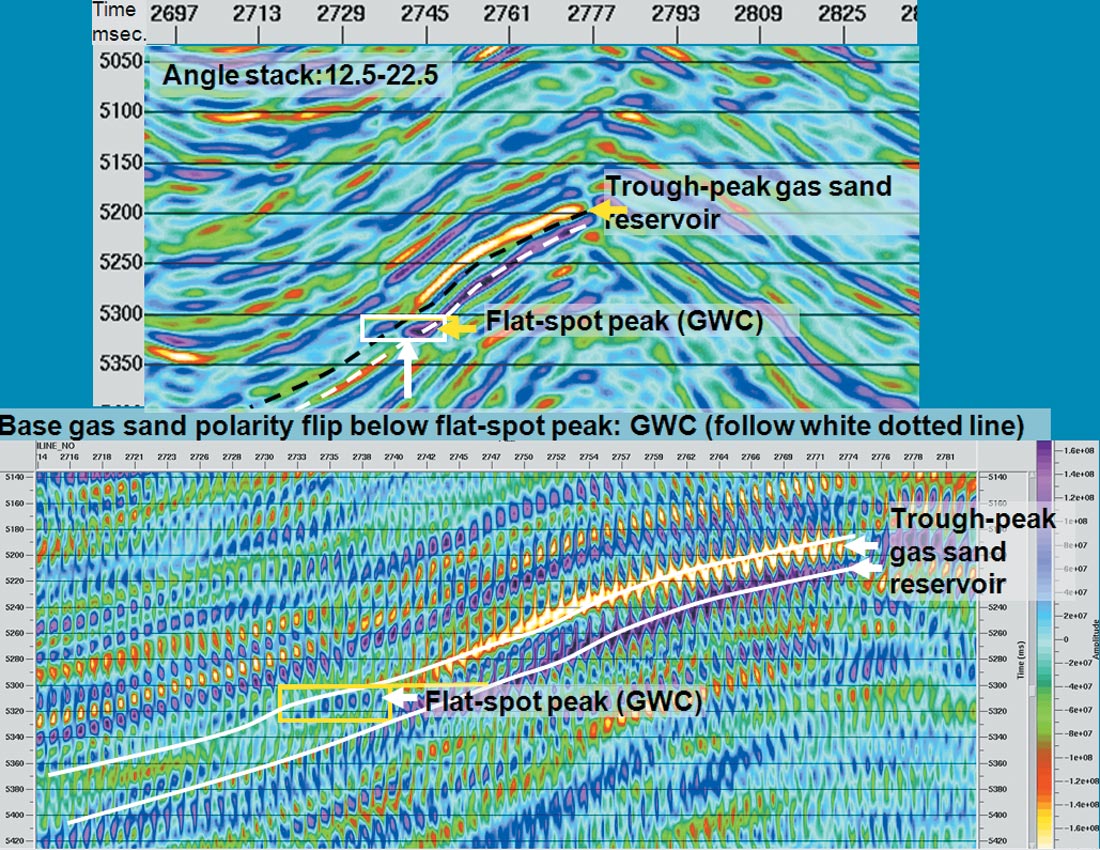
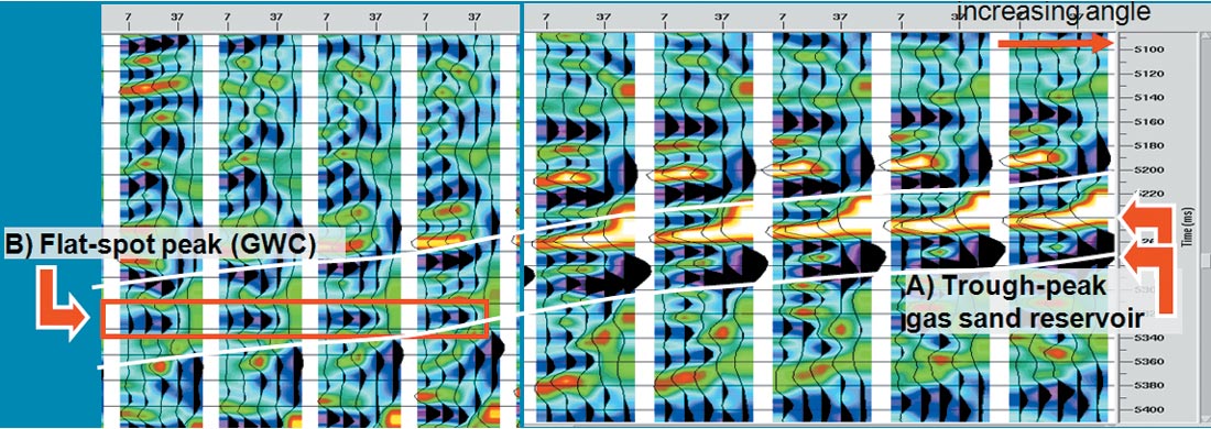
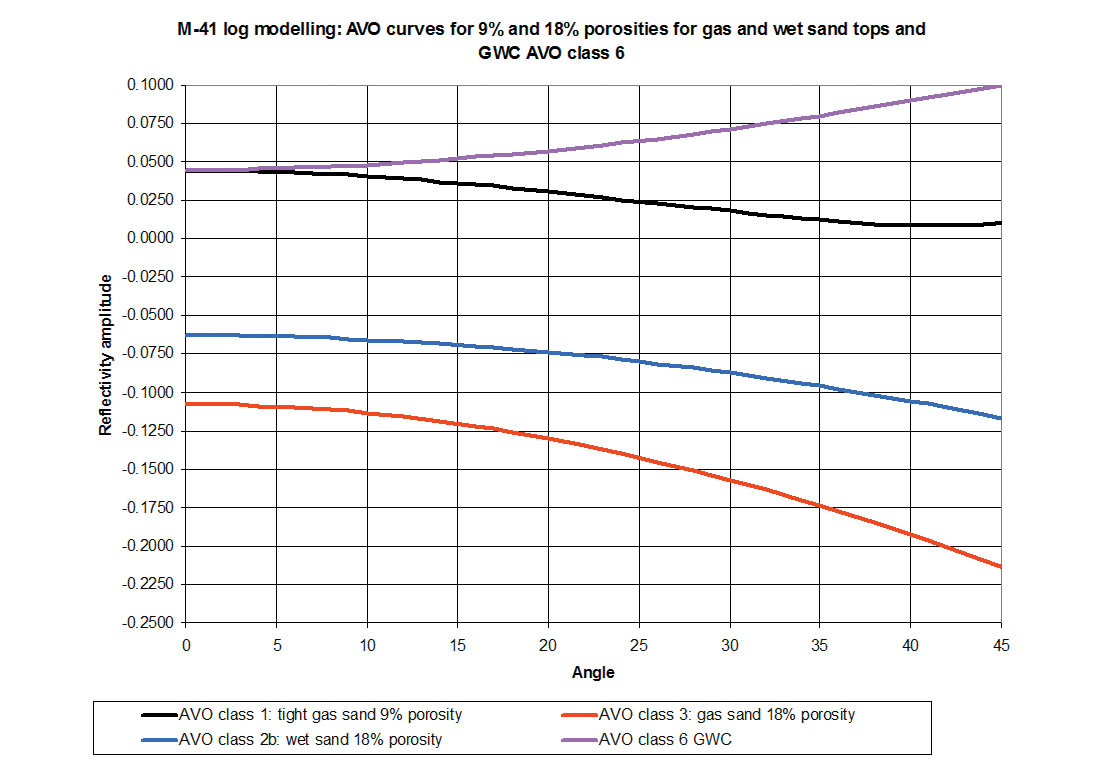
The AVO/LMR fluid and porosity modelling described above facilitated both the calibration and prediction of economic gas sand reservoir. Subsequent pre-stack attribute inversion of the final PSDM gathers confirmed the flat-spot as being theoretically consistent with the new AVO class 6 classification of a true fluid contact down-dip from a strong conventional bright AVO top gas sand trough anomaly seen in the compressed gather display in figure 14. Closer scrutiny of the angle gather stacks for the postulated DHI in figure 14, shows significant brightening with offset for the trough-peak pair (red arrows at Ain figure 15a) updip from the post-stack flat-spot location shown in the red box marked B (GWC) within the white top/base sand horizons in figure 15a. This AVO class 3 response matches the synthetic model response shown in figures 8 and 9b for an 18% porosity gas-saturated sand. Furthermore critical confirmation of the AVO class 3 up-dip gas sand response, is provided by the correct AVO class 6 response of a weak Rp intercept and slight positive gradient (red arrow at B) also shown in figure 15a. Figure 15b shows the various AVO class 3, 2b and 1 curves for a single top sand reflector, representing shale/gas, shale/oil and shale/brine respectively from the M-41 FRM and porosity modelling. A GWC AVO class 6 curve shown in pink is included for comparison and further confirmation of the observed AVO in the red box marked B in figure 15a.

Following this encouraging and exacting AVO class 6 requirement, it was decided to use this DHI as a fluid template for the λμρ-AVO 3D data analysis. Based on the AVO/LMR modelling of the M-41 log data, it was found that the best isolation of the DHI could be achieved by cross-plotting λρ−μρ difference versus P-impedance as shown in figure 7, above. This conclusion is corroborated in figure 16a, that compares log to inverted seismic data by crossplotting the combination of log and seismic derived λρ−μr difference vs. P-impedance attributes. The match between inverted seismic and log data points is remarkably good and assured that the resulting 3D volume mapping of gas sand anomalies, selected from various cross-plot polygons shown in figure 16a, would be meaningful.

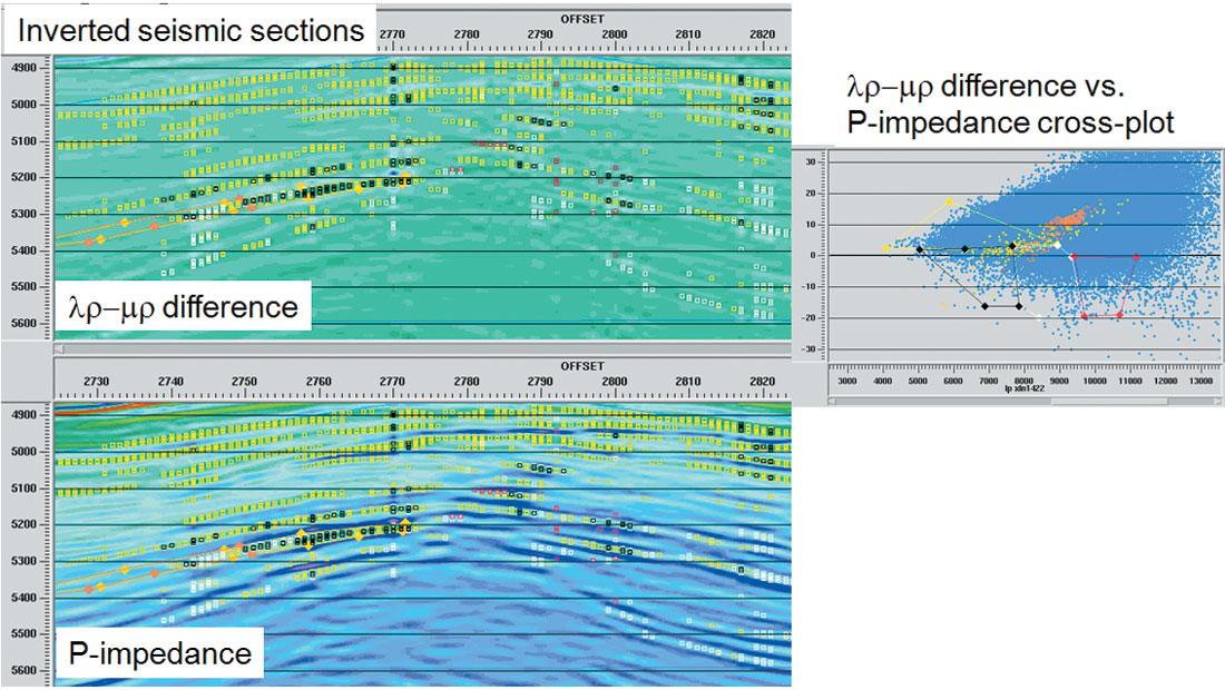
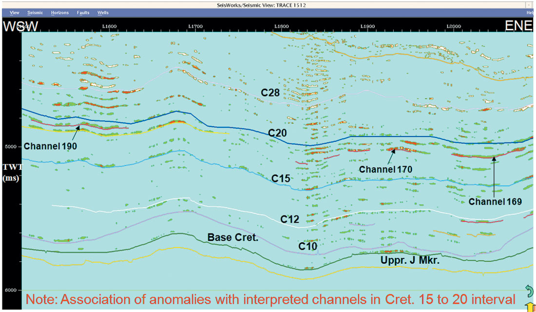
Figure 16b shows the approach used to discriminate gas sands from wet sands and shale background based on a sparsely populated black polygon within this cross-plot space, for the 3D template line through the DHI flat-spot anomaly. The λρ−μρ difference versus P-impedance seismic sections in figure 16b, show black points projected from the black polygon (lower left quadrant) on the periphery of the background shale, which perfectly isolate the bright anomaly originally identified on the stack. Further confirmation of the choice of the black polygon can be seen by the clustering of these black points in a structurally conformable up-dip, crestal position within the postulated gas sand anomaly. Note that the measured values for the known 18% porosity gas sand in the G-24 well also fall within this black polygon thereby adding validity to the choice of these polygon points. Non-prospective shales and wet sands form the majority of the blue cloud to the upper and right quadrants in the cross-plot, some of which have been picked by yellow, white and red polygons shown on the right inset panel in figure 16b. The projection of these points onto the inverted seismic sections encase and surround the black gas sand points, there b y demonstrating the presence of an adequate seal. A specific wet sand orange polygon picked down-dip from the flat-spot on the λρ−μρ difference and P-impedance seismic sections, projects back onto the cross-plot to the upper right, away from the black gas sand polygon as expected from the AVO/LMR log modelling shown in figure 7. The application of these polygon masks to the data isolated other λρ−μρ difference versus P-impedance anomalies throughout a 2D grid of lines selected from the 3D, one of which is shown in figure 17. The association of these polygon mask anomalies with the independent interpretation of channels in the Cretaceous 15 to 20 intervals, adds compelling credence to their validity as DHI’s.

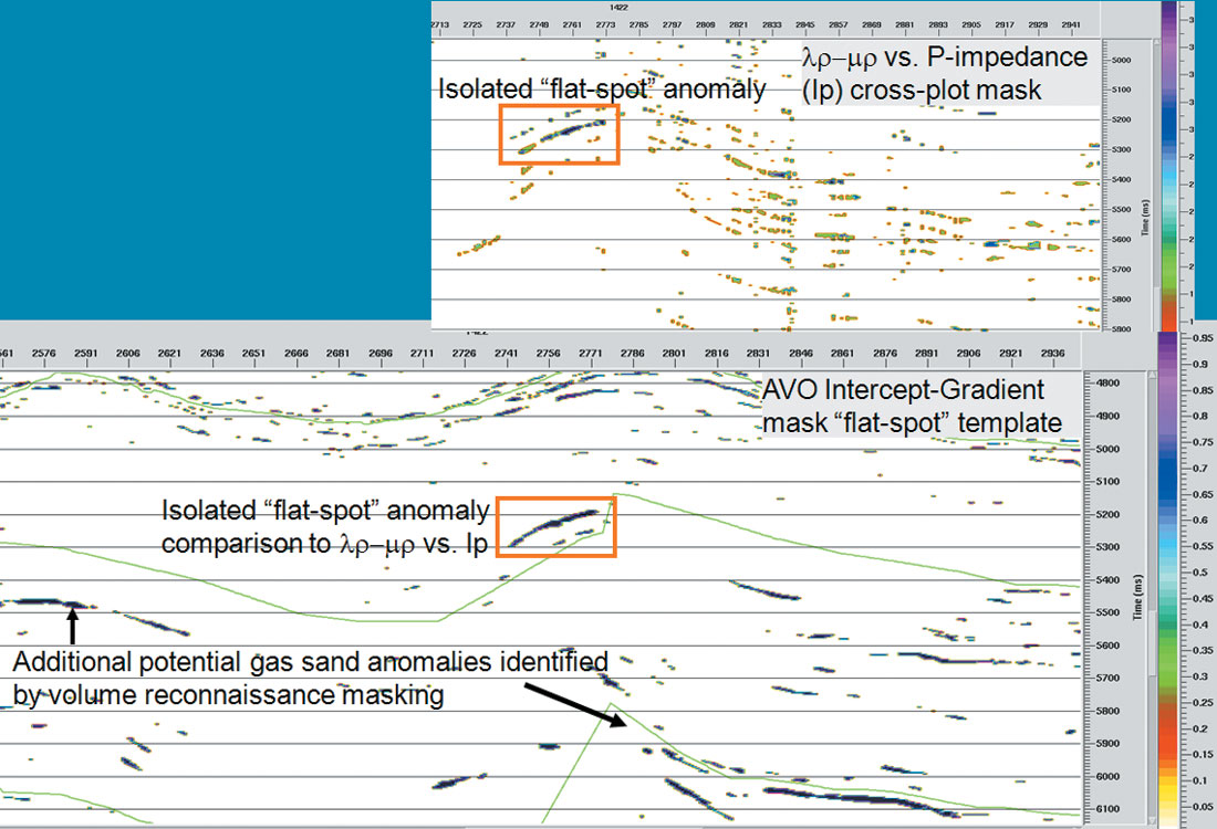
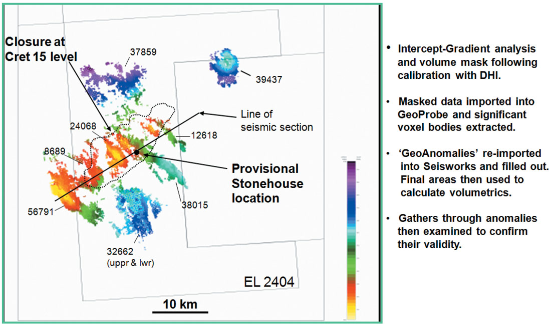
Whilst successful, the λρ−μρ difference vs. P-impedance cross-plot analysis and volume masking was only available for a 2D grid of lines in time. Consequently, driven by the need to utilize the benefit of the full 3D volume in depth, it was decided to see if 3D, AVO intercept/gradient (IG) analysis and volume reconnaissance masking would produce satisfactory results. Again, the DHI flat-spot anomaly was used as a template test. Comparison of the mask results achieved by λρ−μρ difference vs. P-impedance and IG analysis on the flat-spot control, shows that the IG approach satisfactorily isolates the top and base of the gas sand DHI and also provides more discrete anomalies with less spurious attribute chatter as shown in figure 18. A3D, IGbased top/base reservoir sand mask depth volume was subsequently created and imported into GeoProbe for further analysis having identified a number of additional anomalies (see figures 18 and 19).

AVO geo-anomalies were then generated from this masked volume using an appropriate minimum of connected voxels. These were tracked as top and base pairs which corresponded to a trough over a peak, as per the modelled reflection response for a porous, gas-charged sand. As an additional check, gathers through these anomalies were analysed to confirm the ‘correct’ polarity. The geo-anomalies were re-exported to SeisWorks to infill the λρ−μρ difference vs. P-impedance 2D grid and provided a full 3D volume coverage of potential, connected sand channel bodies as shown in figure 20.

The final combined areas were used to help calculate volumetrics for the five target horizons. The reservoir risk element was modified by the assessed quality of the AVO anomalies at each horizon and resulted in a geological chance of success varying from 9% to 27% at the five levels. As a result of the work, the reservoir chance of success assigned to the primary objective interval was increased from 40% to 60%.

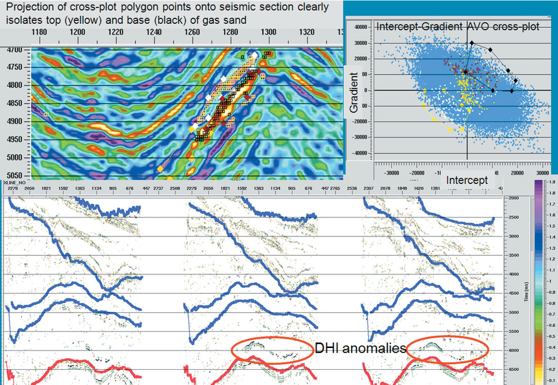
AVO geo-anomalies were then generated from this masked volume using an appropriate minimum of connected voxels. These were tracked as top and base pairs which corresponded to a trough over a peak, as per the modelled reflection response for a porous, gas-charged sand. As an additional check, gathers through these anomalies were analysed to confirm the ‘correct’ polarity. The geo-anomalies were re-exported to SeisWorks to infill the λρ−μρ difference vs. P-impedance 2D grid and provided a full 3D volume coverage of potential, connected sand channel bodies as shown in figure 20.

The final combined areas were used to help calculate volumetrics for the five target horizons. The reservoir risk element was modified by the assessed quality of the AVO anomalies at each horizon and resulted in a geological chance of success varying from 9% to 27% at the five levels. As a result of the work, the reservoir chance of success assigned to the primary objective interval was increased from 40% to 60%.

Conclusions

AVO and LMR analysis has been successful in mitigating reservoir risk at Stonehouse. FRM and porosity substitution work showed that the required high porosity gas sands would produce bright, class 3-4 AVO responses that would clearly distinguish them from the high porosity wet and low porosity wet or gas cases. A DHI with a new AVO type 6 fluid contact was defined and λρ−μρ vs. P-impedance cross-plotting showed that it plotted within the same polygon as the measured 18% porosity gas sand in Annapolis G-24. The anomaly was also successfully isolated using 3D AVO, IG analysis and using this calibration, a top/base reservoir sand mask depth volume was created and imported to GeoProbe for analysis. A significant number of AVO geoanomalies were generated at the objective horizons and used for volumetric and risking analysis. The positive AVO results for the principal Upper Missisauga interval resulted in a significant reduction in the reservoir risk.

Acknowledgements

The authors wish to thank EnCana management for allowing the publication of this material.