Azimuth Moveout Transformation – some promising applications from western Canada

Summary

Azimuth moveout (AMO) is a partial migration operator that rotates the azimuth and modifies the offset of 3D prestack data. Being a wave-equation based re-gridding algorithm, AMO carries the correct kinematic, phase and amplitude transformation, and handles dipping geological strata and variable velocity relatively accurately. These characteristics set AMO apart as a seismic interpolator from conventional techniques. It can also be used to reduce the data size of 3D prestack dataset by coherently stacking traces with similar absolute offsets and azimuths. This work discusses the effectiveness of AMO application on different 3D seismic volumes from western Canada and mentions the advantages that accrue in doing so.

Introduction

It is often found that the offset and azimuth distribution in 3D seismic surveys, both land and marine are sub-optimal, for reasons that vary from practical considerations to economics. Modification of azimuth and offset distributions of data during processing could prove to be an effective method for optimum imaging of 3-D datasets. Introduced by Biondi et al 1998, azimuth moveout is a partial prestack migration process which rotates the azimuth and modifies the offset distribution of the data during processing, without the need for detailed a priori assumptions about the velocity function or geology. The process has been assigned the name ‘azimuth moveout’ (AMO) due to its ability to modify the azimuth of the data.

Though originally AMO was developed to address the shortcomings of marine acquisition, the present day potential applications for the process include the following:

1. Regularization of sparse and irregular geometries

Economic constraints and practical logistics during acquisition of seismic data may cause the data to be sampled in a sparse or irregular fashion along one or more directions. For land data acquisition, physical obstructions and environmental objectives may prevent placement of source and receivers at the desired locations. Extra shots and receivers are also deployed at places that result in sparse coverage at some locations and an overabundance of traces at other locations. For marine data, cable feathering and swath or patch shooting can produce sparse or irregular distribution in offset, fold or azimuth. Irregular sampling may also result from asymmetric shooting geometries and editing of noisy traces.

Various algorithms in the processing stream assume that the physical quantities such as time, source-receiver midpoint, azimuth and offset are continuous. Kirchhoff migration is very sensitive to uneven sampling and can create strong amplitude distortions. Similarly, processes like DMO or algorithms employing any type of Fourier implementation require regular sampling. In reality and for the reasons mentioned above, one or more of these assumptions may not be true.

Wide-azimuth 3-D surveys need an even range of source to receiver offsets at all azimuths and these need to be sampled adequately in space and time. However, in practice, offset and azimuth distribution could vary from bin to bin or could be uniform in say the inline direction and vary in the crossline direction. Significant offset and azimuth irregularities can occur in multi-streamer marine surveys (Chemingui and Baumstein, 2000). If not corrected for properly, these irregularities can not only degrade stacks but can cause amplitude artifacts and positioning errors in the final image, not to mention the fact that they can affect any prestack analysis that may be attempted. Neglecting azimuth variations results in incorrect computation of travel times which enter in to various calculations during imaging, affecting both positioning and amplitude. Conventional binning and interpolation techniques usually ignore the issue of source-receiver orientation and have the detrimental effect of averaging amplitudes over given areas. Application of AMO can transform irregular 3-D surveys with wide azimuthal coverage onto regular midpoint-offset subsets with common source-receiver azimuths. After correction with AMO, the data has the necessary regularization and can be processed using any of the processes mentioned above as well as any of the wave extrapolation methods including finite-differencing and wave equation domain techniques.

2. Reduction of prestack data

One important application of AMO is its ability to reduce the amount of 3-D prestack data, without losing any information by coherently stacking traces with similar azimuths and offsets. Since the kinematics of 3D data depend on azimuths and offsets, the data need to be processed with AMO before stacking, for maximizing coherency among the traces that are averaged. This data reduction would make computer intensive processes like 3D prestack time migration for example, more economical to use.

3. Interpolation of 3D prestack data

AMO serves to be employed for a ‘wave-equation’ interpolation of 3D data to overcome spatial aliasing problems or correct for uneven coverage.

4. Surface-related multiple elimination (SRME)

Matson and Abma, 2005 have recently demonstrated a method for transforming a 2D SRME multiple prediction for marine surveys, to a 3D multiple prediction using AMO for multiples.

AMO process

AMO is defined as an operator that transforms 3-D prestack data with a given offset and azimuth to equivalent data with different offsets and azimuths (Biondi et al, 1998). A process that is somewhat similar (but not the same) to this transformation is DMO, which transforms non-zero offset data to zero- offset data. However, these zero- offset data cannot be properly imaged by prestack depth migration. AMO transforms prestack data onto equivalent nonzero offset data that can be used as input to prestack depth migration. So, Biondi’et al’s AMO formulation is derived from DMO, by starting from the definition of DMO in the frequency-wave number domain (Hale, 1984), and the definition of its inverse (Ronen, 1987). Next, the stationary-phase approximation of the AMO operator expressed in the frequency-wave number domain is evaluated. This yields a time-space representation of the AMO operator that can be applied as an integral operator. This time-space formulation of the AMO operator can now be applied to irregularly spaced data, needless to mention that an accurate implementation of AMO must avoid aliasing of the data and of the operator.

The impulse response of the time-space AMO is a skewed saddle surface – its width and dips are dependent on the values of absolute offsets and azimuths, i.e. difference in azimuths between input and output data. The spatial extent of this saddle increases with the amount of azimuth rotation and offset continuation applied to the data. For small azimuth rotation and offset continuation the AMO operator is compact. In such a case it would be inexpensive to apply. Thus the spatial extent of the operator is maximum for 90 degree rotation and vanishes for offsets and azimuths approaching zero.

A land dataset, with a wide range of azimuths and offsets can be reduced to small set of data-cubes with constant offset and azimuth. Then each of these common-offset cubes can be migrated independently with a 3D prestack migration. The migrated cubes can be stacked together to form the final image.

For more elaborate details about the process, the reader is referred to Biondi et al, 1998 and Biondi and Chemengui, 2001.

Real data applications

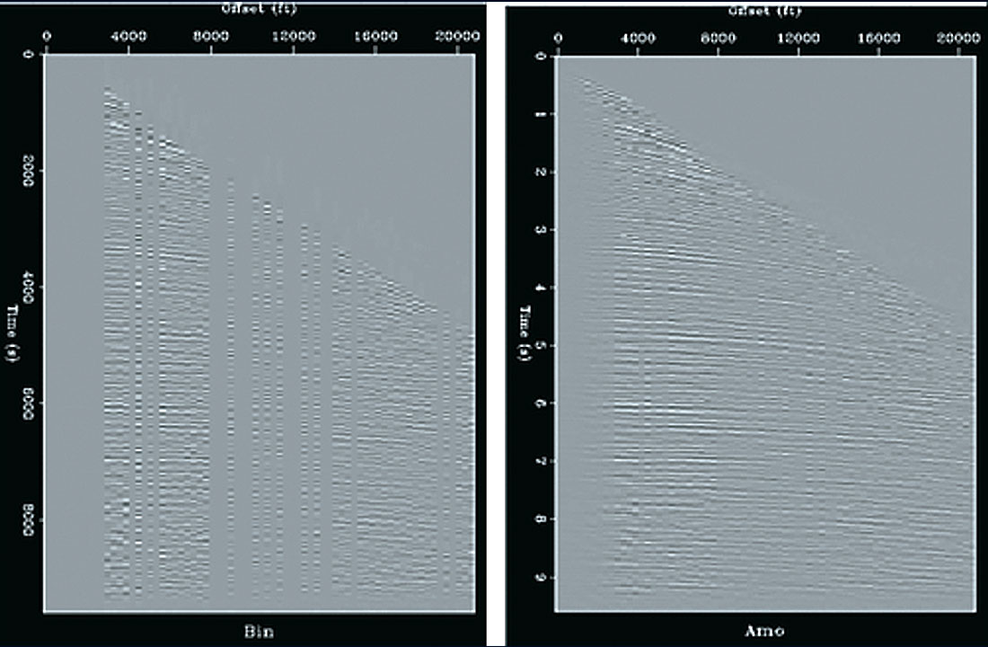
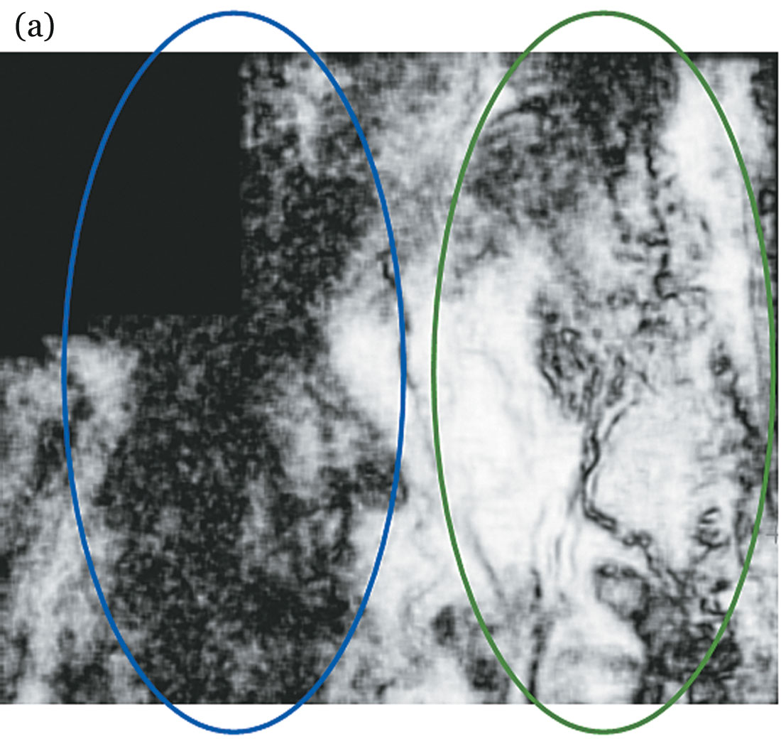
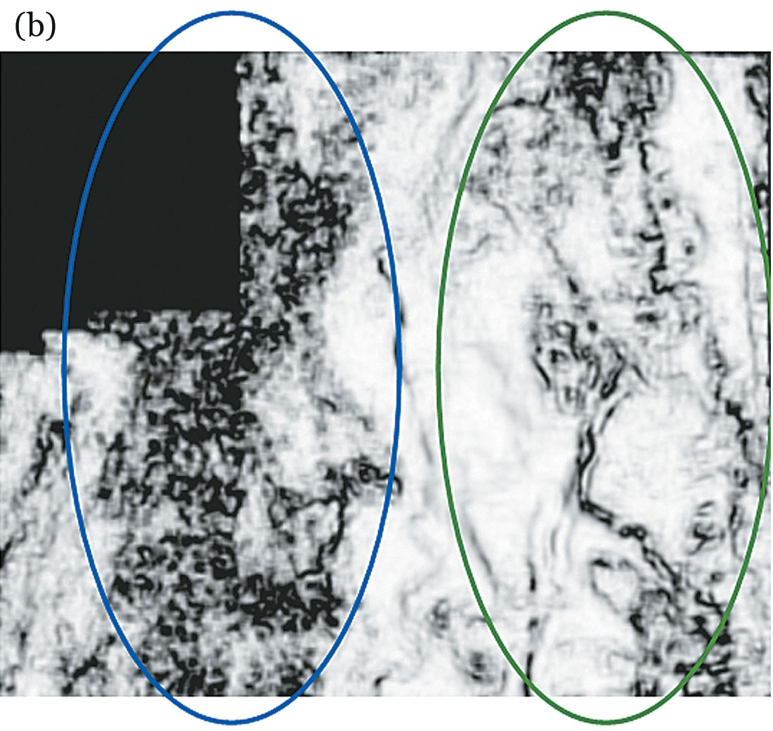
1. As an example of the interpolation of data with AMO, Figure 1 shows two images for a Gulf of Mexico marine data set where missing offsets are filled in during the wave-equation binning process. Notice how the AMO application improves the signal-to-noise ratio and the reflection events look more coherent and so can be easily interpreted.
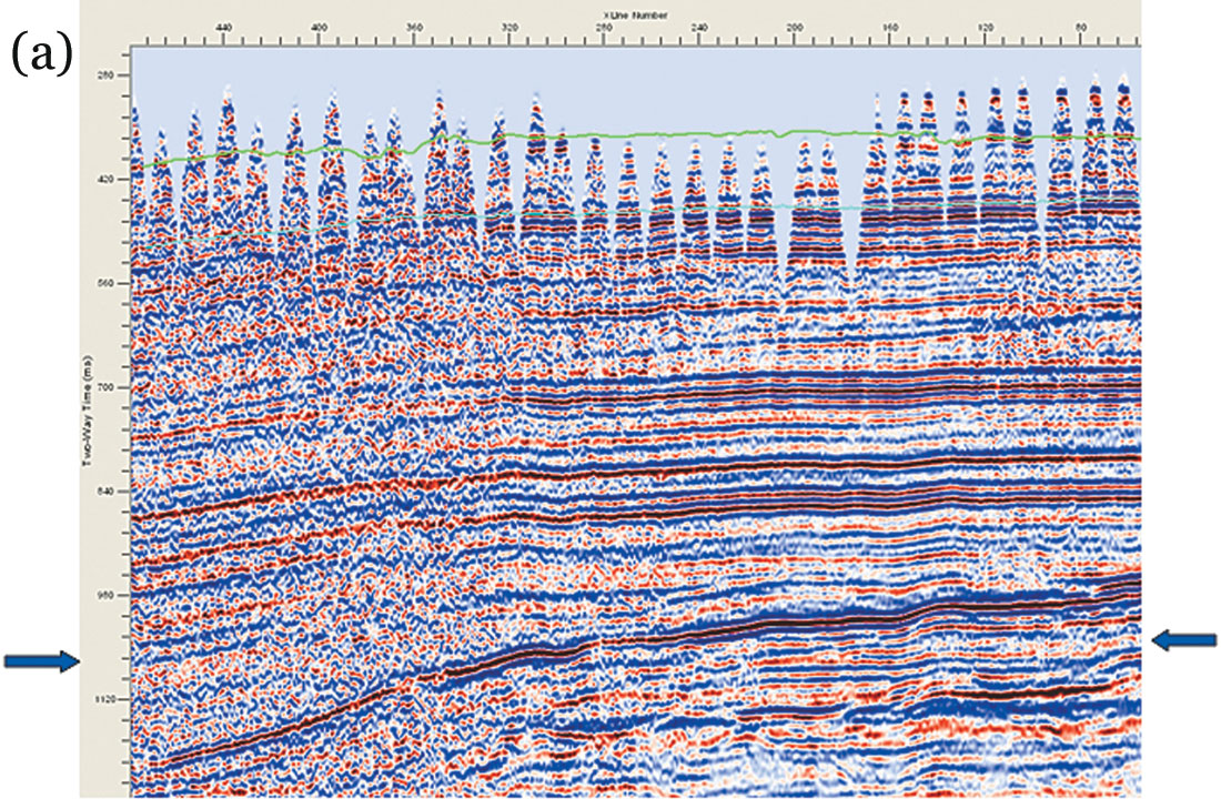
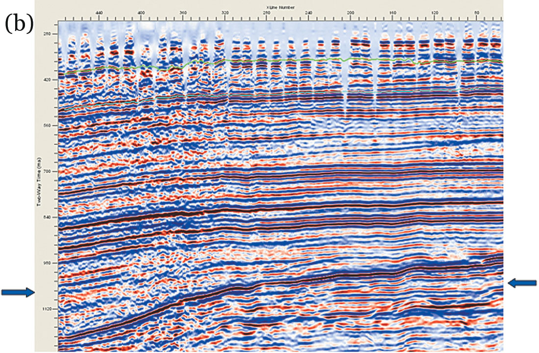
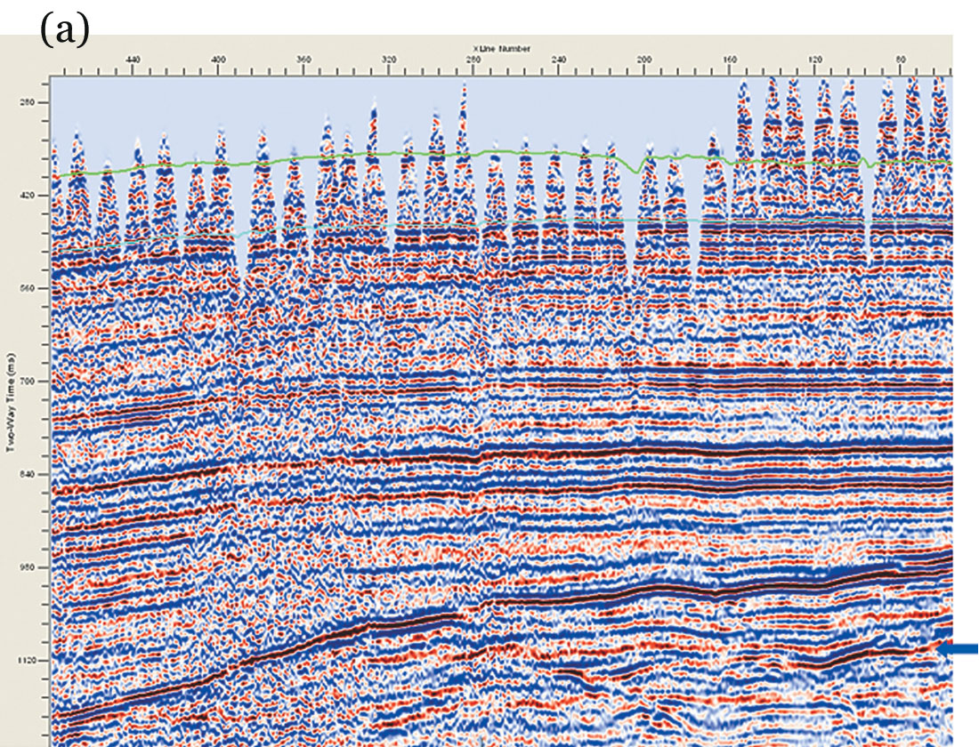
2. AMO was run on different 3-D land data volumes and the effectiveness of the process was evaluated first by visual comparison of the seismic sections and time slices before and after AMO processing. This was followed by comparing coherence displays for AMO application, as it helps in assessing the differences better, due to its high spatial resolution. Figure 2 shows an inline before AMO, from the Winfield 3-D land data set from central Alberta. Notice the gaps in the data in the shallow zone. Also, notice the discontinuous nature of the seismic reflection seen at 360 ms or so (indicated with blue arrows). After AMO application the gaps are filled up and signal-to-noise ratio is also somewhat better. Notice how the main reflection at 360 ms now looks more continuous. The feeble reflections below the main event are also seen more focused and continuous.

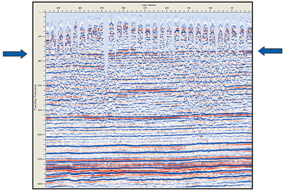
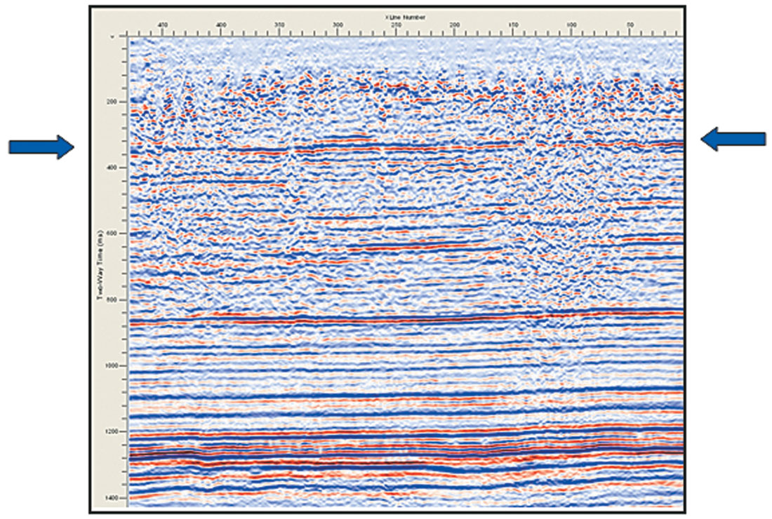
Figure 3 shows a pair of amplitude time slices from the Winfield 3-D seismic volume. Evidently, the AMO application makes the slice amplitudes look more focused and sharp.

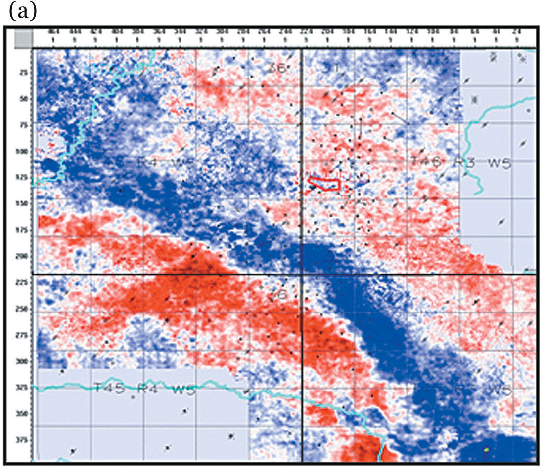
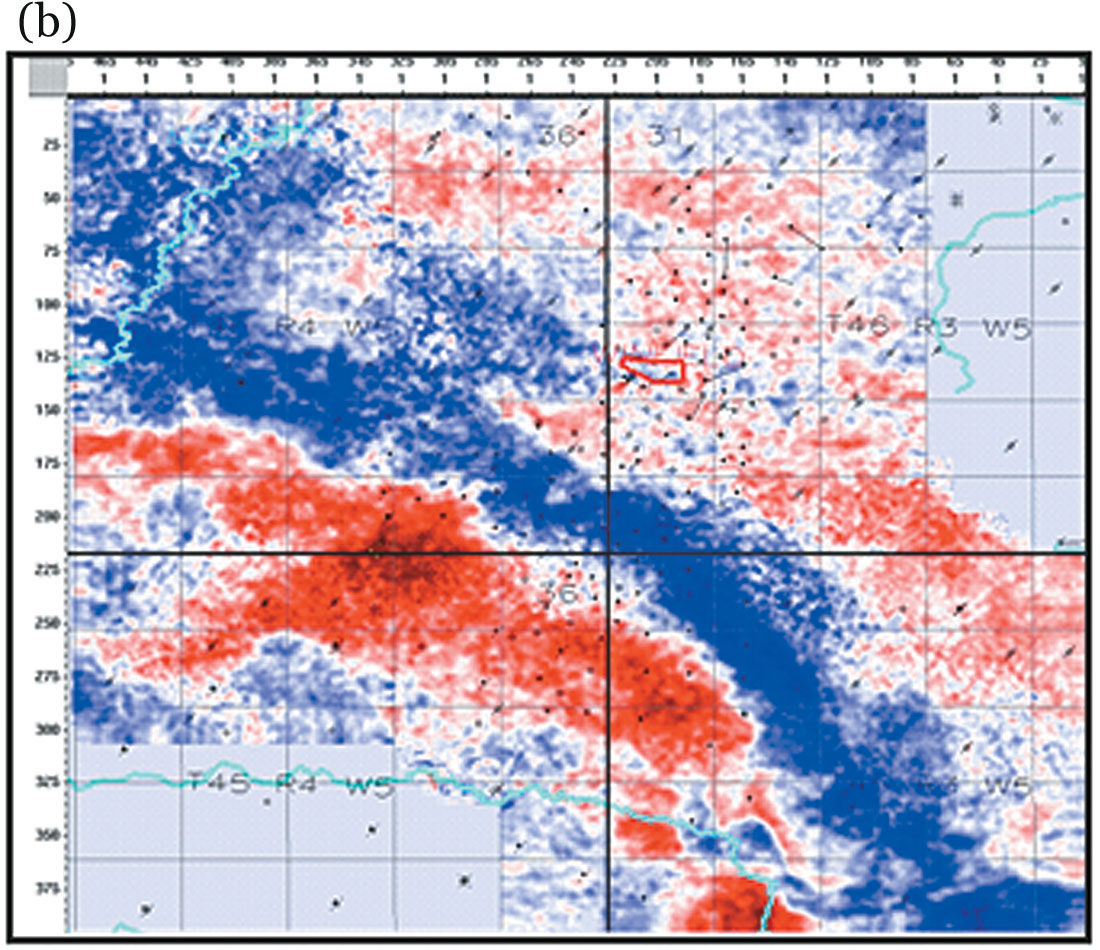
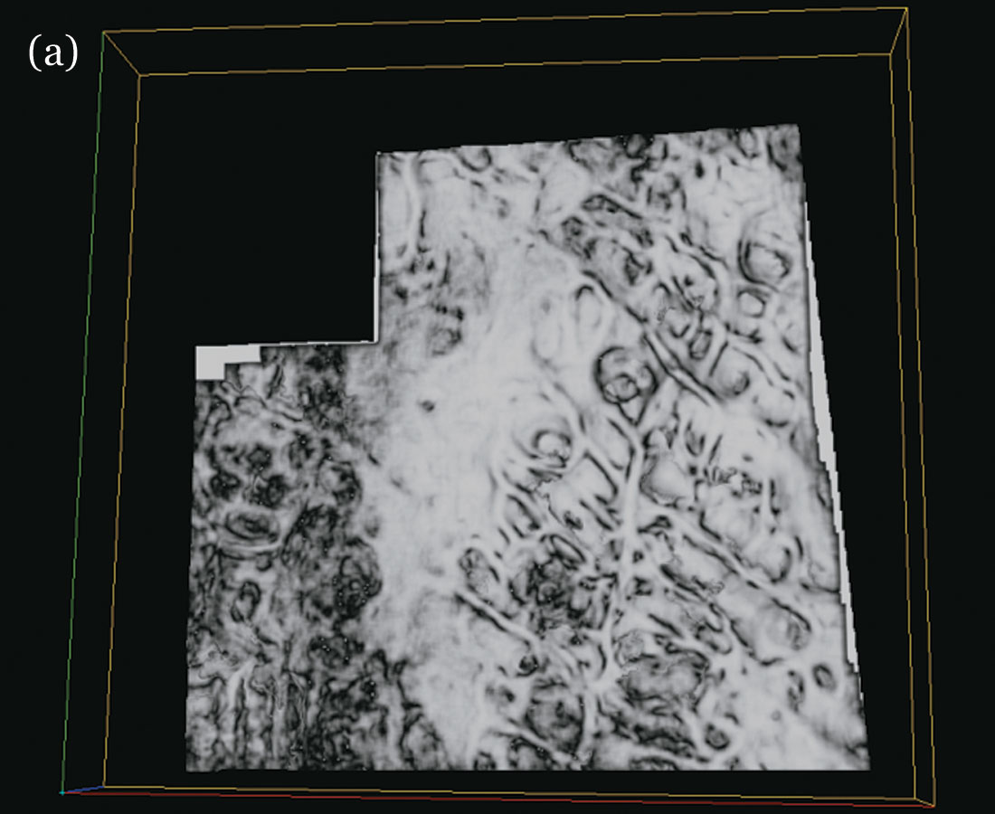
Figure 4 is a pair of coherence time slices (at 320 ms) from the Winfield 3-D volume. Notice the missing data along the receiver lines before AMO processing is filled up after its application. At least two fault trends can now be seen starting from the left, one running downwards and the other going to the right.

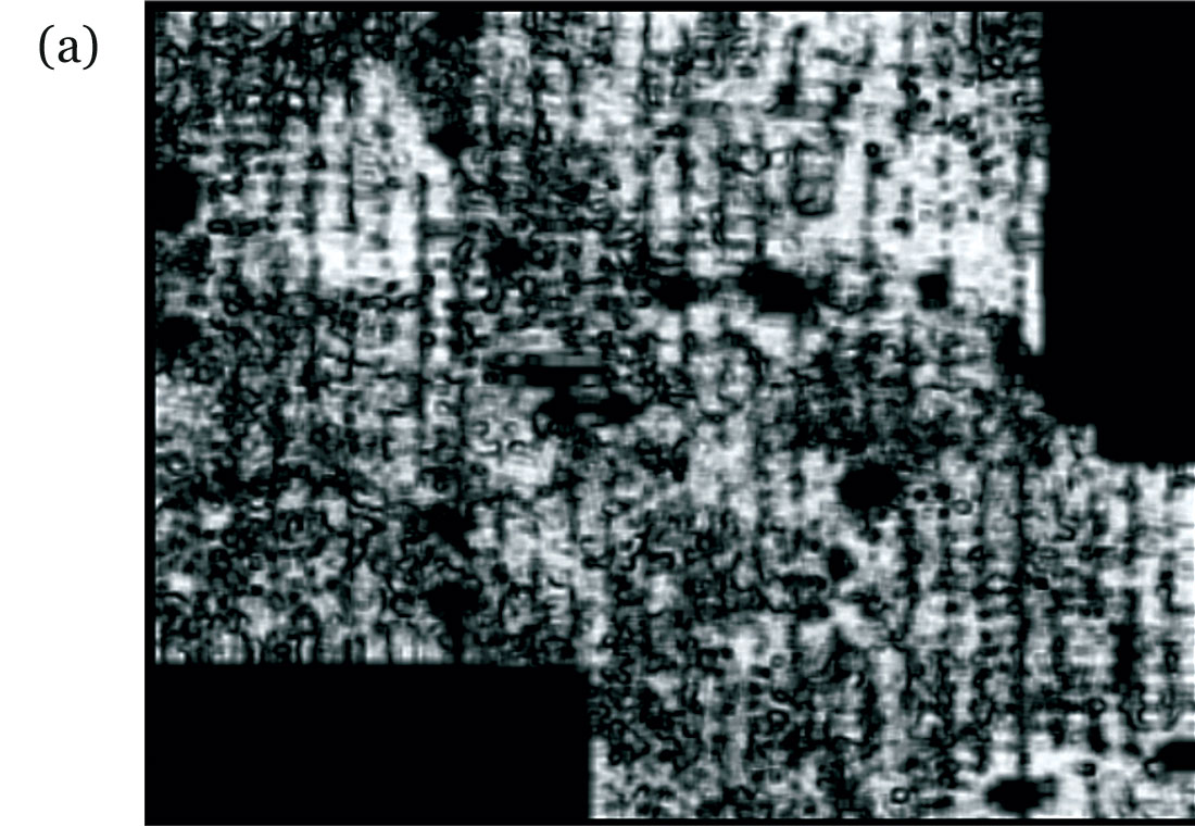
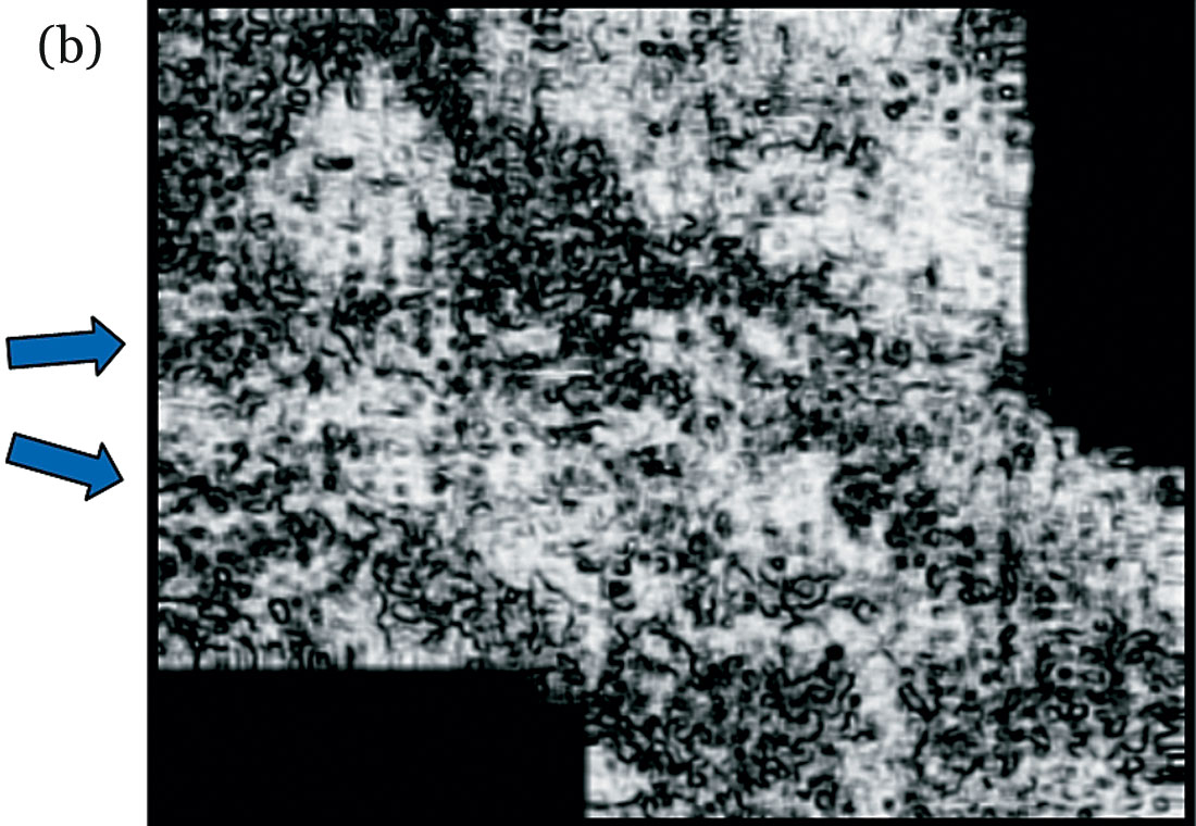
Figure 5 shows another comparison of two coherence slices at 1324 ms from the same Winfield volume before and after AMO processing. In the highlighted zones, the events look sharper, suggesting that apart from the shallow levels, events at deeper levels also benefit from AMO application.

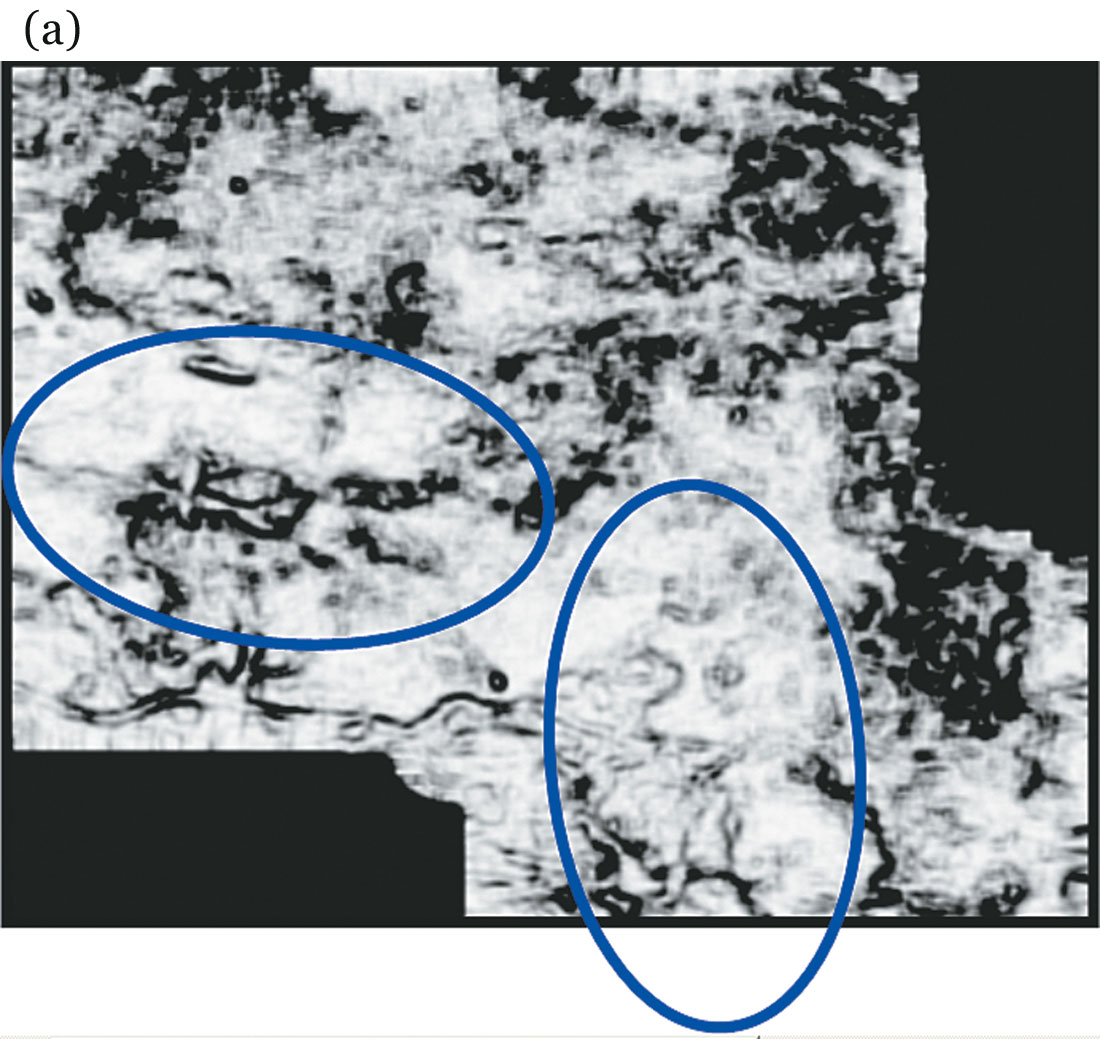
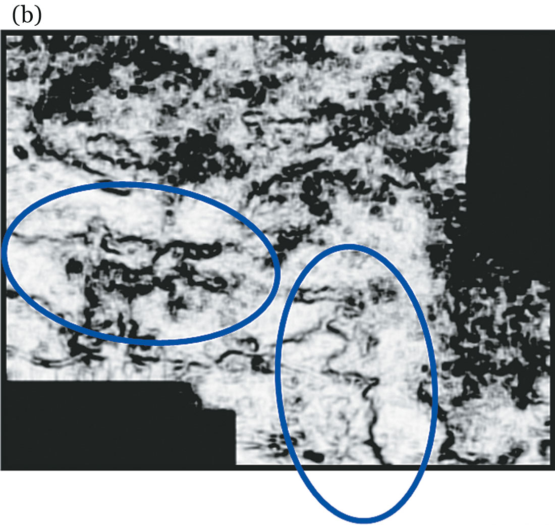
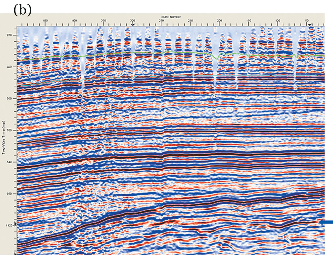
Figure 6 (a) and (b) show a seismic inline from another 3-D volume from Alberta, before and after AMO application. This example shows a pronounced improvement in the overall signal-to-noise ratio after AMO. Also, notice how the missing data gaps get filled up after AMO application and the reflections look more coherent and amenable for better interpretation. A set of coherence time slices at 1018 ms corroborates the above conclusions. The low coherence features to the left on figure 7 appear less noisy. The definition of events in the highlighted zone appears to be much better after AMO application.

Another set of inlines from the same volume are shown in Figure 8 (a) and (b). Again, better signal-to-noise ratio, filling of missing data gaps and more coherent reflections can be seen after AMO application. A pair of coherence strat-slices at the level indicated (arrow) on the inlines in figure 8, are shown in figure 9. All the events are now well defined and so the interpretability of seismic data is definitely improved.

Conclusions

The effective offset and azimuth of 3-D prestack data can be modified during the processing flow, with the application of AMO operator (partial migration operator) to the prestack data. The method addresses proper handling of irregular geometry and therefore allows for reliable pre-stack analysis (AVO) analysis of migrated data. Improved signal-to-noise ratio and coherency of reflection events, and features showing up crisp and distinct on time or strat-slices after AMO processing, leads to enhanced interpretability of post stack seismic data.

Acknowledgements

The authors are grateful to the personnel (especially Samo Cilensek), involved in AMO processing of the data at Arcis Corporation, and to Arcis Corporation for the support, permission to use the data examples, and to publish this paper.