Avoiding pitfalls in geostatistical reservoir characterization: A survival guide

I. Introduction

Geostatistics provide a powerful framework for combining sparsely sampled but accurate well information with the densely sampled but less precise 3D seismic information. When used correctly it can provide accurate estimates of reservoir properties and an assessment of the uncertainty and risks associated with our reservoir models. However, geostatistical tools can be easily abused when the assumptions underlying the use of these tools are violated. Neglecting geology and geophysics reduces geostatistics to a purely statistical process that may give us false confidence in spurious results. The question that we are trying to answer is: How can geoscientists and reservoir engineers know whether any particular reservoir characterization project, using geostatistics and seismic attributes, is valid or whether it is an abuse of the geostatistical techniques? This article will attempt to answer this question by illustrating the potential pitfalls of the method and proposing actions to avoid them. In addition, we will recommend a set of key information that should be included with all geostatistical projects to allow other geoscientists and engineers to assess the quality of the results.

We will focus our discussion on the geostatistical technique known as collocated cokriging. Collocated cokriging is a geostatistical mapping technique, based on kriging and linear regression, that honors the petrophysical information derived at well locations and the spatial trends of related seismic attributes. It is probably the most popular geostatistical technique for combining petrophysical and seismic information. We will take a detailed look at potential pitfalls and problems that can occur in each of the key steps of a cokriging study and make recommendations on how to avoid these problems. Many of these observations are applicable to other geostatistical techniques that combine wells and seismic data. We will also list the information that should be recorded in a final report that will allow other geoscientists and engineers to make a proper assessment of the study.

II. Practical Guidelines and Potential Pitfalls

Most geostatistical reservoir characterization studies share a number of common elements. These elements are best introduced in the context of a small case history. The objective of this study was to create a net sand thickness map on the basis of the interpreted well log data and the 3D seismic interpreted horizons.

A. Assessing data quality

Case study

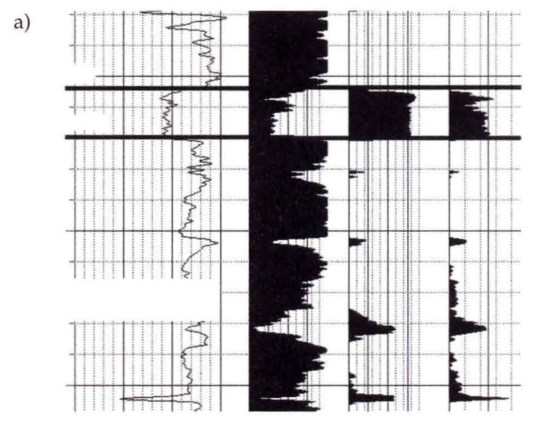
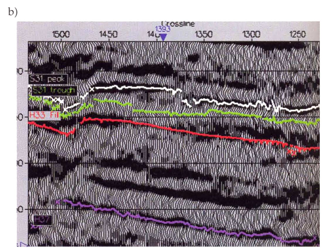
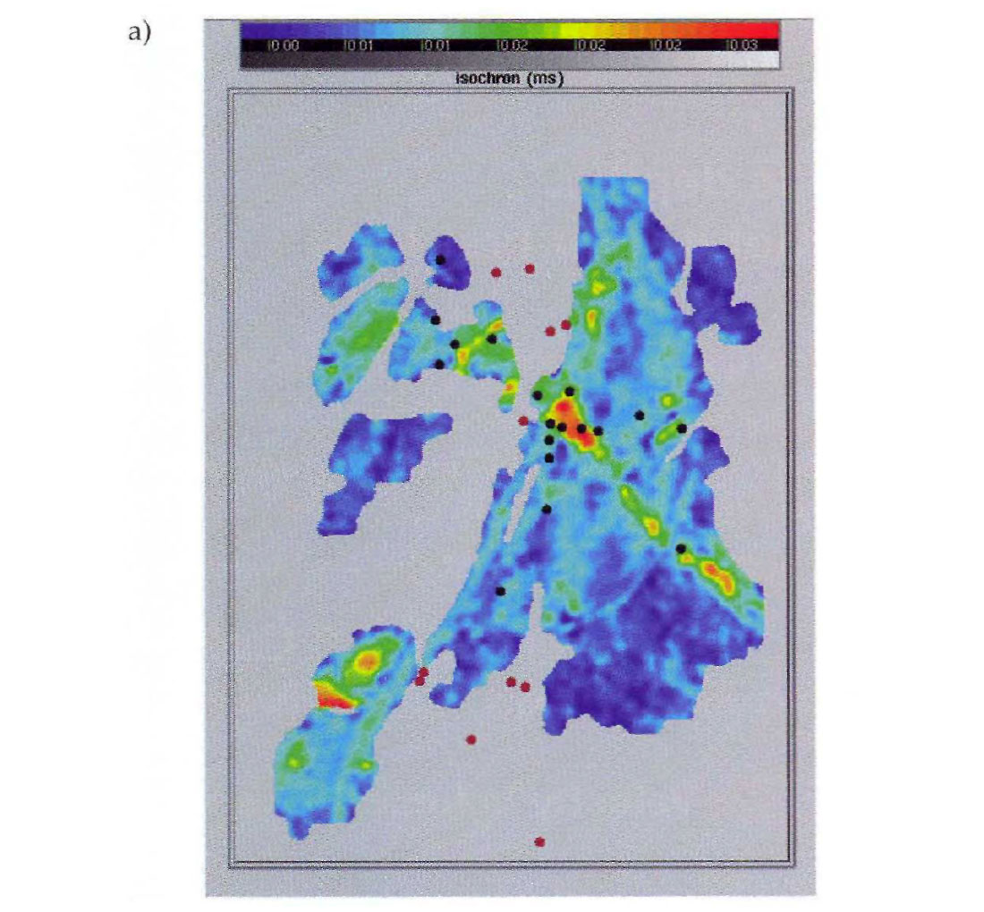
The first step in our geostatistical study consisted of gathering all of the data and familiarizing ourselves with the geological and petrophysical reports and the interpreted seismic sections. Seismic and well information for this study are shown in Figure 1. Sand thickness had been previously calculated for each well in the study, based on the interpretation of petrophysical logs. The top and bottom of the reservoir had been interpreted on the seismic data and the resulting isochron time thickness correlated strongly with the well-log derived estimate of sand thickness at the well locations.

General discussion

Gathering and assessing the necessary data is a major and important step in all reservoir characterization studies. It is important to remember that poor quality seismic and/or well log data can only result in a poor reservoir characterization and the data used in modelling should always be weighted according to it's reliability.

Well log information is generally considered to be "hard" or accurate data in geostatistical modelling because the measurements are made in the formation with a variety of tools that are directly related to the reservoir properties of interest (i.e. bulk density is linear, porosity weighted combination of matrix density and fluid density). However, it is important to remember that problems can exist with the well log data. In many cases the well logs have been acquired over a number of years. Changes in logging tool response or log processing parameters (like water resistivity, matrix density, clean sand and shale baselines, etc.) can cause an artificial bias in the petrophysical parameters. This bias can seriously degrade the calibration between well and seismic data. In most cases the petrophysical properties are averaged to provide a single value of porosity (or other parameters) for the reservoir zone. This averaging, often performed with interpretive cut-off values applied, can greatly impact the well to seismic calibrations.

Seismic data is considered to be "softer" or less reliable than well log information because the seismic measurement is made remotely and it is only indirectly related to the reservoir properties of interest (i.e. amplitude is proportional to reflectivity which is proportional to the changes in acoustic impedance which is proportional to density, etc.). Even seismic data that is of generally high quality can have localized problems with noise, multiple contamination, acquisition footprints, poor stacking or migration velocities, etc. In most cases the seismic attributes used in reservoir characterization are extracted from the 3D seismic volume along interpreted horizons. If the interpretation is not correct the attributes could be meaningless.

If the data quality is not good, a geostatistical study is probably not warranted.

B. Initial data analysis

Case Study

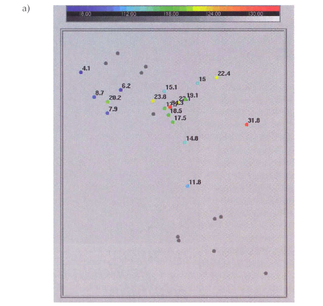
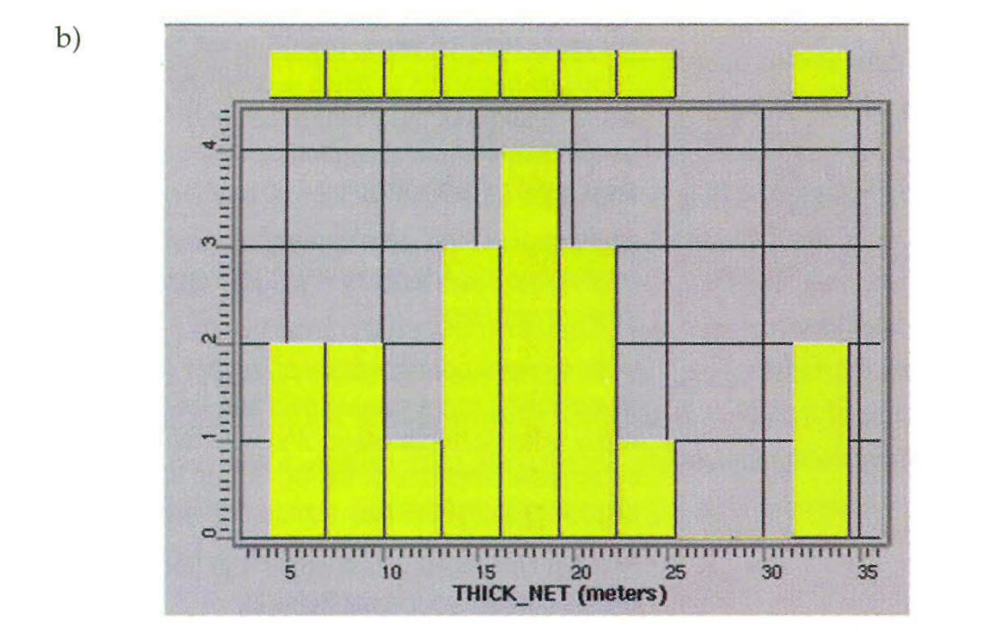
The next step in our study was to review the statistical behavior of the data in the context of the geological and geophysical model. We posted the net sand information from the wells on a basemap (Fig.2a) to a look for spatial trends, and we generated histograms of sand thickness from the well information (Fig. 2b) to assess the average, range, and distribution of sand thicknesses found at the existing wells.

General discussion

Geostatistical reservoir characterization often involves the exploration of large and complex data sets. Time spent reviewing the petrophysical and seismic information at the beginning of the project is an important investment. This allows the geoscientist to become familiar with the data, to determine whether the data and the relationships between well and seismic data are valid, and to recognize anomalies early in the study. Most of the geostatistical processes make assumptions about the statistical distribution of the reservoir properties. While the techniques are robust it is important to insure that the data are consistent with these assumptions. The data should also be viewed in the context of a geologic model because this should guide the choice of tools used in geostatistical mapping.

Several factors should be considered during the data analysis phase. The first is to assess the quality and consistency of the data. One method of checking the data is to generate histograms of the reservoir and seismic parameters. Several geostatistical procedures are based upon an assumption of Gaussian or normal distribution and this can be recognized as the familiar bell-shaped curve on the histogram. Unfortunately, the data distribution for well-derived parameters is often difficult to assess because the sample sizes are small and sampling is biased so the distribution must be inferred. If the parameter values tend to be skewed towards the high or low end of the range or if multiple peaks are present in the distribution, this could be a sign of non-stationarity or a non-normal distribution.

Histograms should also be examined them for outliers. Histogram outliers (or univariate outliers) are one or more data points (but generally not more than a couple) that are clearly separated (by more than 2 or 3 standard deviations) from the rest of the data. Outliers can have a major impact on spatial correlation modelling and on the correlation between seismic attributes and petrophysical properties. Individual wells or areas of the seismic data that appear to be anomalous should always be checked and verified. If the outliers represent poor data quality or mistakes in interpretation or processing, they should be removed from the analysis. However, it is important to consider that outliers can represent points from another population of data, caused by changes in lithologyor fluid content. If the outliers represent a different population of data, they must be dealt with separately, but they cannot be simply removed without affecting the estimation /simulation process.

Statistical sampling is one of the most serious problems in a typical study. Geostatistical mapping applications assume that the mean and variance of the reservoir properties derived from the well locations are representative of the entire field. This assumption is almost always violated because wells are drilled for a specific objective (produce maximum amounts of hydrocarbons) and not to sample the statistics of the reservoir. For example, if a field was discovered on the basis of seismic bright spots, then areas of low amplitude are typically not drilled. Wells are more often drilled on the structural highs than lows. While all of these practices make sound economic sense, they bias the statistical sampling of the reservoir. One way of dealing with this type of problem is to add "pseudo wells" that represent the potential non-economic reservoir parameters to balance the statistics of the field. These added control points are interpretive and should be created with geologic guidance. Interpretive decisions of this nature should always be thoroughly documented in the final report.

Statistical stationarity is one of the most important assumptions in geostatistical mapping. In short, this is the assumption that the statistics (i.e. mean and variance) of the population (reservoir) are consistent throughout the study area. One common cause of non-stationarity is the existence of a trend across the field. Regional dip is a common example of this problem. This type of non-stationarity can be easily diagnosed by calculating the mean value of the reservoir property in different areas of the field or by cross-plotting the reservoir property against the coordinate data. These trends should be estimated and removed from the data prior to mapping and added back afterwards.

Changes in lithology, facies, or fluid saturation are another common cause of non-stationarity. These variations often lead to distinct statistical populations in the reservoir. For example, the average porosity in a sand-filled channel facies is usually very different from the porosity in the adjacent shales. If wells from the channel sands and the shales are treated as a single population the variance would be overly large and the average value of porosity could be completely unrepresentative. This type of non-stationarity can be difficult to recognize, especially when few wells are available. If it is not taken into account, the mapping results can be very misleading. Coding wells by facies type, fault block or fluid type is an important step in determining if this type of non-stationarity is a problem. Statistical parameters, such as mean, variance and regression coefficients can then be estimated independently within each group.

When this type of non-stationarity is present, it is necessary to subdivide the data into separate populations before beginning the analysis and mapping within each group or facies type independently. This will be discussed later in the cokriging section.

C. Calibrating the seismic attribute to the reservoir property

Case Study

In our study we found a strong correlation between the seismic isochron time and sand thickness at the wells. This high correlation was supported by a definitive physical relationship; thicker sands relate directly to longer travel times ( provided the velocities remain reasonably consistent). Because of this correlation, the seismic isochron map (Fig. 3a) clearly provided additional information about the variation of sand thickness in the interwell space (areas of the field where the sand was not present were not mapped on the seismic data). However, even in this ideal case, 4 of the 22 wells did not follow the main regression trend (Fig. 3b). This was a clear indication of non-stationarity, or multiple populations in the data. Closer examination of the interpreted horizons in the vicinity of these wells indicated that the seismic data were miss-picked due to a crossing channel system. At this point the ideal solution would have been to correct the seismic interpretation and repeat the analysis. Unfortunately, the seismic response in the area of the crossing channels was complicated due to interference between events and we could not interpret the event with confidence. This left us with a difficult problem. How could we honor the strong correlation trend present on the majority of the wells and still accept that there would be uncertainty in our maps due to the complications with the seismic interpretation? First we chose to estimate the regression line and correlation coefficient from the 18 wells that followed the main trend.

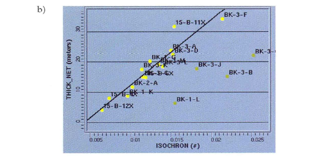
This regression line intersects all 18 wells and the correlation coefficient ( R ) between seismic isochron time and sand thickness was estimated as 0.94. Next we estimated the regression from all 22 wells and estimated a correlation coefficient ( R ) of 0.60. This lower correlation coefficient was more representative of the uncertainty in the seismic interpretation but the corresponding regression line did not intersect any of the wells. Our goal was to honor the regression line from the 18 wells with the uncertainty estimate from all 22 but the regression slope was directly related to the correlation coefficient. We analyzed the regression equation and found that the standard deviation of the seismic isochron could be realistically increased to reflect the added uncertainty in the seismic picks and this increase in the standard deviation, together with the decrease in the correlation coefficient, resulted in a regression line that honored the main trend. Ultimately, many of these decisions were interpretive and all of this information was detailed in the final report.

General discussion

The most common approach of finding seismic attributes that correlate with reservoir properties is purely empirical. The interpreter generates a number of attribute maps from the seismic data around a single horizon or between two horizons. The attribute values at the well locations are extracted from the maps and crossplotted against the reservoir properties of interest. Cross plots and bivariate statistics are used to determine how well the seismic attributes correlate with the reservoir properties. Since this is a purely statistical approach the geoscientist should strive to discover a reasonable deterministic explanation for the correlation. Usually this can only be done with the help of seismic modelling and rock physics information.

Modem software packages have greatly simplified the task of extracting seismic attributes and of generating crossplots of seismic attributes versus reservoir properties. This practice has become wide-spread in the industry in recent years however there are several pitfalls.

1. Sampling the seismic attribute data at well locations

As mentioned earlier, it is necessary to sample seismic attributes map at the well locations. A common practice is to select attributes values where the well intersects the seismic horizon(s). However, the well locations may be mis-positioned with respect to the seismic attributes because of navigation errors, seismic migration errors, well bore deviations and other effects. Geologic effects, such as facies changes, faults, and discontinuities degrade the correlation if the well is not correctly positioned with respect to the seismic. In general, if the number of wells is plentiful, attributes can simply be chosen at the well locations since random errors in the seismic attributes will average out. However, if the number of wells is sparse, then the errors in the attributes may not average out or the results may be biased, and the location of the wells with respect to the attributes becomes more critical.

Creating forward synthetics from the sonic and density logs and correlating these synthetic traces with the seismic traces near the corresponding well locations can help determine which seismic trace location is most representative of the underlying geology (Boerner et at 1997). The seismic traces selected for attribute extraction will be at the locations which provide the best match between the synthetic and seismic traces. If several traces provide good matches, the seismic attributes from these trace locations can be averaged together to provide an attribute value for the well. Deviated wells provide additional challenges for extracting seismic attributes.

When random noise contaminates the seismic data the correlation between the seismic attributes and reservoir properties can be improved by smoothing the attribute data prior to sampling at the well locations. Specially designed moving average windows can also be used to remove seismic acquisition artifacts. The practitioner should use this tool with caution. Attribute windows can have an almost infinite combination of shapes, sizes, and weights applied to each of the attribute locations within the window. With all of these combinations, there is real danger in generating a window that will maximize the correlation between the smoothed attribute and the reservoir property of interest when there actually is little correlation between the two variables.

2. Interpreting cross plots

One of the key tools that is used in calibrating seismic attributes with reservoir properties is the crossplot. It is a visual representation of the relationship between the seismic attribute (the independent variable) and the reservoir property of interest (the dependent variable). The practitioner can use the crossplot to visually identify outliers that may bias the correlation, detect if the relationship is nonlinear, identify different trends which may indicate multiple populations within the dataset, and gain a visual sense for the strength of the correlation between the two variables.

The most common problems are associated with interpreting correlation coefficients. The standard correlation coefficient R (Pearson correlation coefficient) is a measure of the linear dependency of the two variables. The value ranges from 0 (for no correlation) to +/- 1 (perfect positive or negative correlation). It is important to remember that correlation coefficient estimates have uncertainty associated with them. The smaller the sample's size, the greater our uncertainty about what is the true correlation between the two variables.

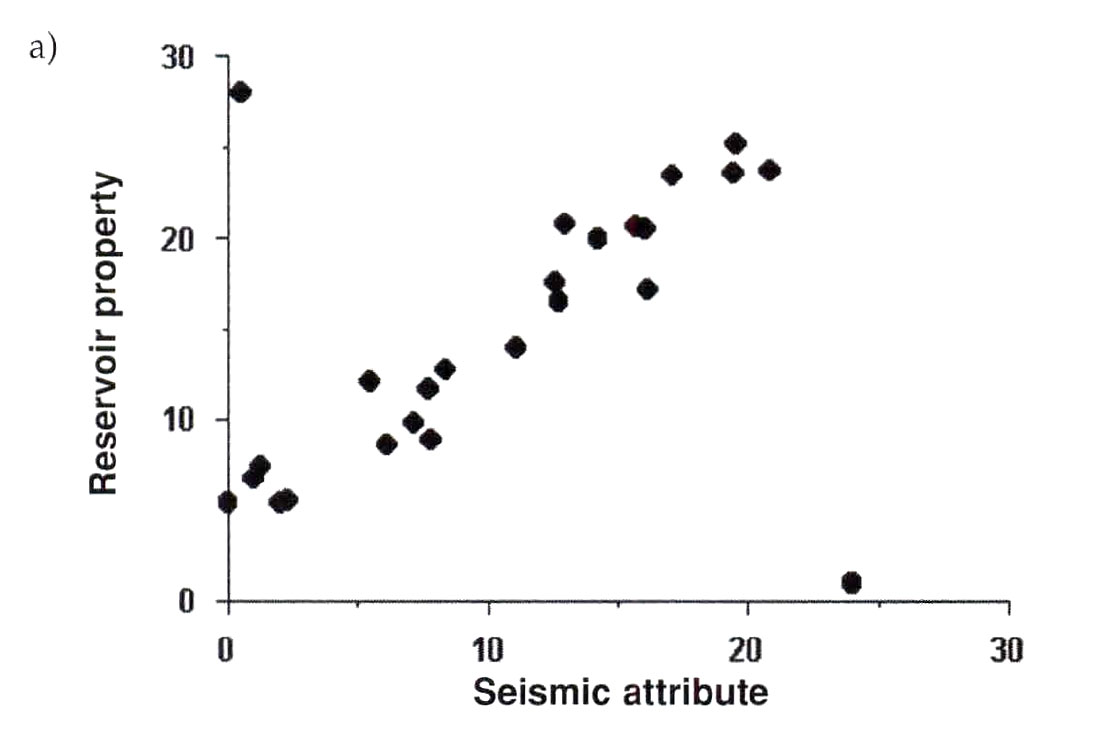
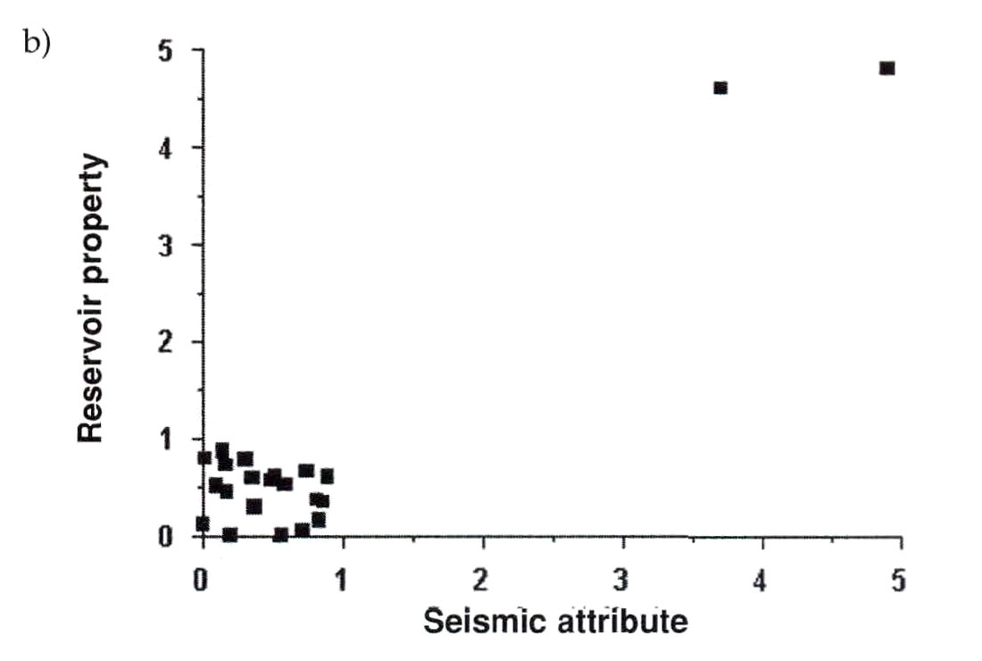
When considering the value of correlation coefficients it is important to check the data for outliers. We already discussed outliers in the earlier section on histograms (univariate outliers) but outliers on crossplots (bivariate outliers) plot away from the regression trend, rather than the average of the single variable. Univariate and bivariate outliers are not always the same points. It is certainly possible to have univariate outliers that fall on regression trends with correlated variables and it is possible to have bivariate outliers that fall within the main distributions of both the dependent and independent variables. Outliers can have a dramatic effect on the correlation coefficient in either direction as shown in the following examples. Figure 4a shows a cross-plot with a seismic attribute plotted against a reservoir property for 25 wells. The correlation coefficient along the central trend is greater than 0.9; however, the effect of 2 outlying wells reduces the apparent correlation to 0.44. With all 25 wells included, the 95% confidence limits on the regression slope range from 0.068 to 0.805. The opposite example is shown in Figure 4b where a cross plot of seismic attribute versus reservoir property is shown for 22 wells. The correlation coefficient in this example is 0.93 but this value comes almost entirely from the two outlier wells. Their effect on the correlation coefficient was examined by first calculating the correlation coefficient with the outliers present, and then removing the outliers and calculating the correlation coefficient again. The correlation coefficient after removing the outliers reduced to -0.22. In reality there was no significant correlation between the two variables. When outliers exist, the practitioner should determine the reasons for the outliers if possible. Some of the causes for outliers are:

• Different populations of data (Non-stationarity)
• Errors in the seismic or log interpretations
• Noise in the seismic or log data
• Variations in the phase and amplitude spectra of the seismic data
• Coordinate data for seismic and/or well data within the area is incorrect

In most cases, unless the cause of the outlying values can be corrected, they should be removed. However, outliers may represent a second population, or legitimate extreme values in the data volume. Plots of the well and/or seismic attributes displayed on a basemap or cross-section can reveal a spatial pattern or trend, which would indicate non-stationarity. This could be caused by saturation changing from water to gas, amplitude changes caused by tuning, changes in lithology, etc. In these situations, it can be important to use the information from the outlier wells; however, regression relationships based on outliers should never be used directly unless the relationship can be supported with seismic modelling.

Finally, all judgments regarding outliers are interpretive in nature. These decisions should be noted in the final report, along with the graphs to support the decisions. For example, if the practitioner has determined that the outliers represent spurious samples that should be removed from the database, this should be noted in the final report. Crossplots generated before and after outlier removal should be a part of the final report as well as the relevant bivariate statistics, such as the estimate of the correlation coefficient, and the linear regression equation that relates the seismic attribute and the reservoir property of interest.

3. Spurious correlation

Spurious correlations (or apparent correlations between two uncorrelated variables) are a serious problem in relating seismic attributes to well data. In general, as the number of seismic attributes increases, the probability of a spurious correlation between at least one of the seismic attributes and the reservoir property of interest will increase. For example, if one had 10 independent well observations, was seeking a correlation coefficient ( R between a seismic attribute and a reservoir property that had an absolute value greater than 0.6, and was searching through 10 seismic attributes, then there is a 50% probability that at least one of the seismic attributes would have a sample correlation coefficient ( r ) greater than 0.6 even when there is actually no correlation between any of the seismic attributes and reservoir property. In other words, because of the large number of attributes considered, there is a 50% chance of observing a correlation coefficient ( r ) of magnitude 0.6 or greater when there is actually no correlation between the reservoir property and the seismic attributes.

4. Assigning physical meaning to the seismic attribute correlation

In general, seismic attributes that are directly related to the reservoir property of interest are the best candidates for geostatistical modelling. Seismic travel time, isochron, and amplitude are good examples of these attributes. Inversion converts seismic traces to estimates of acoustic impedance which is physically related to porosity, lithology and saturation. When more abstract seismic attributes are correlated with the well information, it can be very difficult to assess whether the observed correlation has a physical meaning, or whether it is purely a product of chance. Seismic attribute maps should always be included in the final reports.

Confidence in the correlation with seismic attributes is related to the number of independent measurements of both the seismic attribute and of the reservoir property. If the practitioner has a few wells, there is substantial uncertainty in any correlation. However, if one has many wells, the confidence in a significant correlation increases.

Seismic modelling can be an important step in calibrating seismic attributes with reservoir properties when few wells are available. Existing wells can be modified to reflect a range of geologically plausible changes in reservoir thickness, lithology, porosity and fluid saturation. Synthetic seismic traces can be generated from these "pseudo-well" control points to simulate a larger geological sampling. The seismic interpreter can extract the same seismic attributes from these synthetic seismic traces as are derived from the real seismic data. In the case of the synthetic traces, the relationship between the extracted attributes and the reservoir parameters is already known. If trends from the real seismic data follow the correlation trends observed between the same attributes in the model data then the seismic attribute data can be used with confidence.

5. Assessing the risk and value of using seismic attribute correlations

In some cases, where: 1) there are a large number of wells (for example > 60), 2) there is a large absolute value in the correlation coefficient between the seismic attribute and the reservoir property of interest (say 0.8), 3) the crossplot between the seismic attribute and the reservoir property of interest is linear, and 4) the correlation is not unduly influenced by outliers, there is enough empirical evidence to confirm statistically that the seismic attribute and the reservoir property are related. In these cases, it may not be crucial to understand the physics underlying the relationship.

When the number of wells is small or the number of seismic attributes is large relative to the number of control points, it is more important to validate that there is a physical reason for the correlation. There is one exception to this rule. If the cost of using the seismic attribute and being wrong is small compared to the benefit of using the seismic attribute and being right, then it is advantageous to use a seismic attribute. This situation may occur in exploration situations. If however, the cost of using the seismic attribute and being wrong is high compared to the benefit of being right, (as in the case of development) it is often better not to use the seismic attribute unless the correlation can be explained.

6. Assessing the statistical value of the regression relationship

When we perform multiple linear regressions of one or more independent variables to predict a dependent variable, we use a least squares technique which linearly relates one or more independent variable(s), x, such as our seismic attributes, to a dependent variable, y, such as our reservoir properties. Because the linearity assumption, any nonlinear trends must first be removed before performing the regression. Examination of the crossplots of each independent variable versus the dependent variable will reveal if any of the relationships appear to have a definite nonlinear trend. If a nonlinear trend is found, it is usually possible to create a transform of that independent variable such that the transformed variable is linearly related to the dependent variable. It is always best, if possible, to transform the independent variable rather than the dependent variable to remove non-linearity.

We would like to know how well our regression model will predict, given a new value of x, x_i , not in our original dataset. In essence, we are performing an experiment. We have used a least squares algorithm to build a regression model which explains a relationship between one or more independent variables (seismic attributes) x, and a dependent variable (reservoir property of interest) y. One way to assess how well the regression model will predict future values is to find the 95% confidence interval for the predicted value of y, ŷ_i , at a new value of x, x_i. That is, we can find the minimum and maximum values that are expected to bracket 95% of the actual values of the reservoir property associated with a specific seismic attribute value(s).

You can find the equation for forming this confidence interval on a predicted value of y for given set of x values in any textbook on regression. The maximum and minimum values found from this equation will be centered about the predicted value of y. The distance of the maximum and minimum values from the predicted value of y depends on: 1) how confident we wish to be that the actual y value will be between the calculated minimum and maximum, 2) how large our sample size is, and 3) how far the new x value is from the mean x value. For a 95% confidence interval minimum and maximum will represent the 2.5% percentile value and the 97.5% percentile value. Note that use of the confidence interval equation assumes that the prediction errors (residuals) are uncorrelated and normally distributed with zero mean. If you have not removed any nonlinear trends, these assumptions will not be true.

The confidence level and the confidence bounds (minimum and maximum) should be included in the final reports.

D. Spatial correlation analysis

Case study

We performed spatial correlation analysis of the sand thicknesses derived from the wells using a directional correlogram. Two azimuths were analyzed and fitted with an analytical model (Fig. 5a). The analytical model is required for the geostatistical mapping procedures. Unfortunately, the well information did not provide adequate spatial sampling for the correlogram analysis. Because the seismic isochron and measured sand thickness are highly correlated, we were able to generate a more robust spatial correlation model from the seismic isochron map (Figs. 5b and 5c).

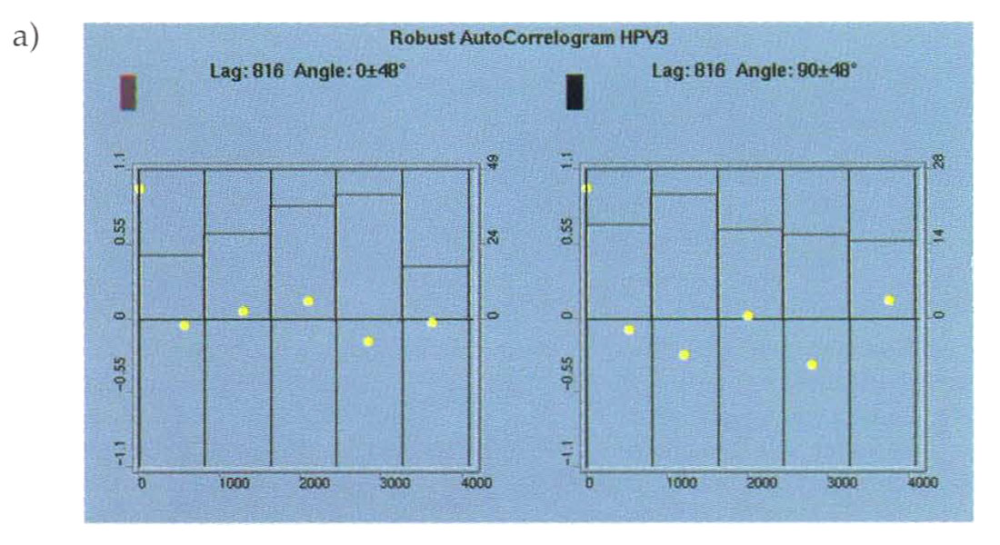
General discussion

Spatial correlation modelling differentiates geostatistical mapping from conventional mapping techniques. The spatial correlation model allows the practitioner to impose geological trends on the mapping process, and it also provides the basis for uncertainty analysis. Unfortunate!~ in many cases a representative spatial correlation model cannot be reliably derived from the limited well data. Another serious problem occurs when the well spacing is large compared to the spatial variation of the reservoir properties. In this case, the reservoir property appears uncorrelated in the spatial correlation analysis and the selection of a spatial correlation model is largely interpretive. Several plausible spatial correlation models should be carried forward through the study to incorporate the uncertainty of this parameter.

Correlograms of seismic attributes that are correlated with the reservoir property can sometimes help in confirming the anisotropic correlation trends in the data. However, seismic data is inherently averaged and it will not provide representative estimates of reservoir property variability over short distances. Outcrop information from similar depositional settings may be helpful in deriving better correlogram estimates for the near distances. When the spatial correlation model has been derived, it is important to compare it to other sources of geological trend information such as the direction of dominant sediment transport.

Extreme or outlier data points can have a very strong effect on the spatial correlation analysis and these should also be removed prior to modelling. Spatial correlation modelling has several assumptions that can be violated in some geological environments. Traditional spatial correlation techniques assume that there is one dominant trend in correlation over the entire field. Many geological environments are not consistent with this assumption. In the case of meandering channel systems, for example, it is important to estimate the spatial correlation in the paleo-flow direction and vary the direction of the correlation model to reflect changes in flow direction.

The spatial correlation model is the foundation for most of the traditional geostatistical uncertainty analysis. Kriging and cokriging error maps are directly derived from this model and the variance in stochastic simulation is also controlled by this parameter. The sill value is directly related to the variance that is expected in the final maps of the reservoir property. Therefore it is important to consider whether the variance estimated from the existing wells is representative of the range of property values across the entire field. The spatial correlation model should always be included in the final report along with documentation of the decisions made in choosing the model.

E. Mapping from the wells alone (Kriging)

Case study

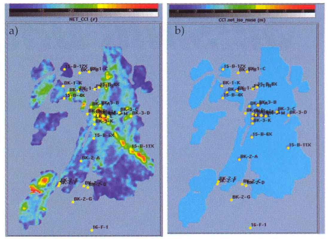
We used simple kriging to create sand thickness maps from the well information (Fig. 6a). This map does not look geologically plausible (with smoothly interpolated sand thickness and bulls eyes around well locations), because the spatial correlation length is less than the average interwell distance. The map is still useful because it gives the gross trend of the thickness variations and provides a useful comparison to the cokriged model. The associated kriging error map (Fig. 6b) does not give quantitative information about the expected uncertainties because it is based upon a statistical model chosen for the mapping. However it helps to assess the relative quality of the interpolation in different areas of the map.

General discussion

Kriging estimates reservoir properties in the interwell space using a weighted average of the property values at the existing well locations. The kriging weights are derived directly from the spatial correlation model. It is often helpful to generate kriged maps prior to performing more sophisticated geostatistical mapping to get a representative view of the trends in the reservoir parameters.

Cross-validation, the technique of sequentially removing each well from the kriging analysis and estimating the property value on the basis of the other wells, should be used to assess the prediction value of the method. The interpolated map, error map, and cross-validation results from kriging should be included in the final report for comparison to the cokriging results.

F. Mapping from seismic and well information (cokriging)

Case study

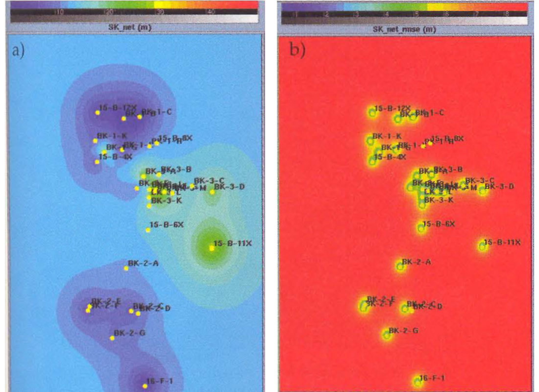
We used collocated cokriging to create a new map of sand thickness based on well and seismic derived information (Fig. 7a). This map and the associated error map appear to be more consistent with the geological model than the kriged results. A cross-validation analysis indicates that cokriging had much lower prediction error than kriging due to the inclusion of the seismic information Wells that were not included in the regression analysis have larger prediction errors because they include sand thickness values from the deeper channel together with the primary reservoir.

General discussion

Cokriging provides a means of including seismic derived information in the geostatistical mapping process. Collocated cokriging can be shown to be a linear combination of kriging from the wells alone and linear regression. Kriging ensures that the final maps will honor the well information and linear regression reduces error away from the wells through inclusion of the seismic attribute data. Cokriged maps, along with the associated error maps should be included in the final reports for comparison to the kriged maps. Cross-validation should also be performed and tabulated to assess the prediction accuracy It is often useful to compare the cross-validation from cokriging to the cross-validation derived from kriging and linear regression.

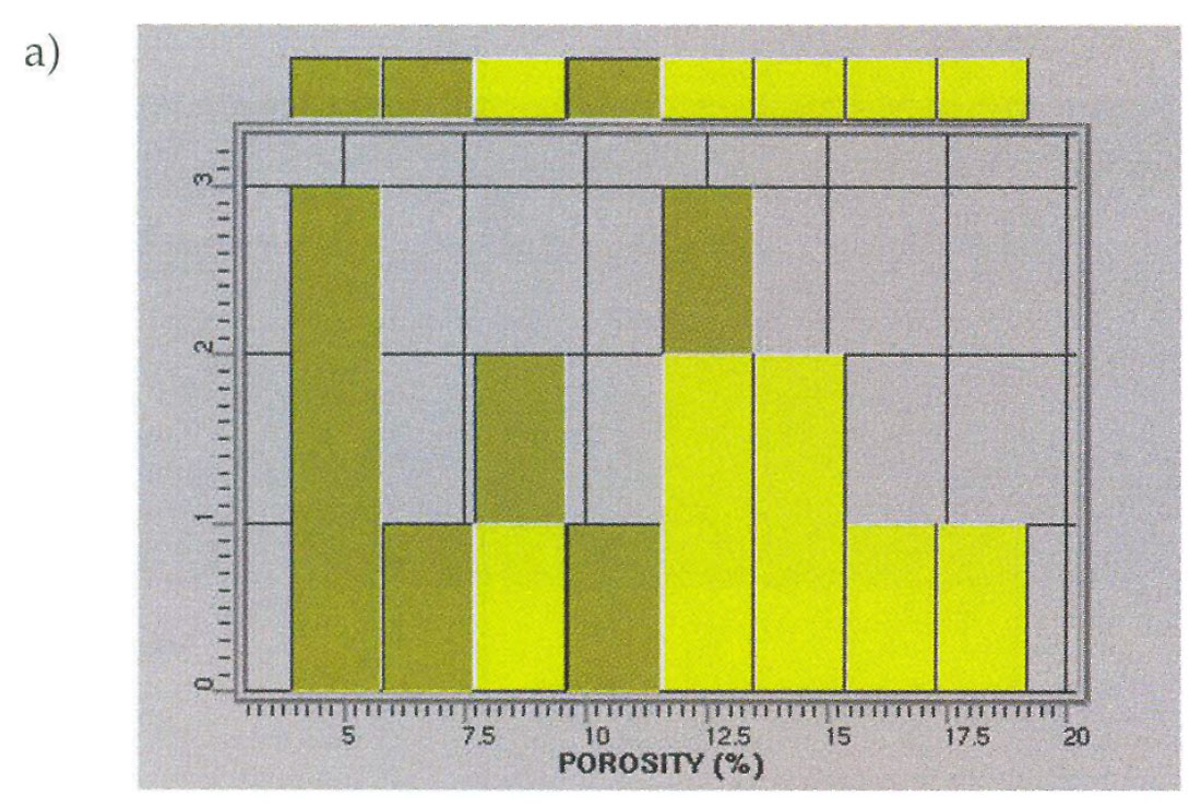
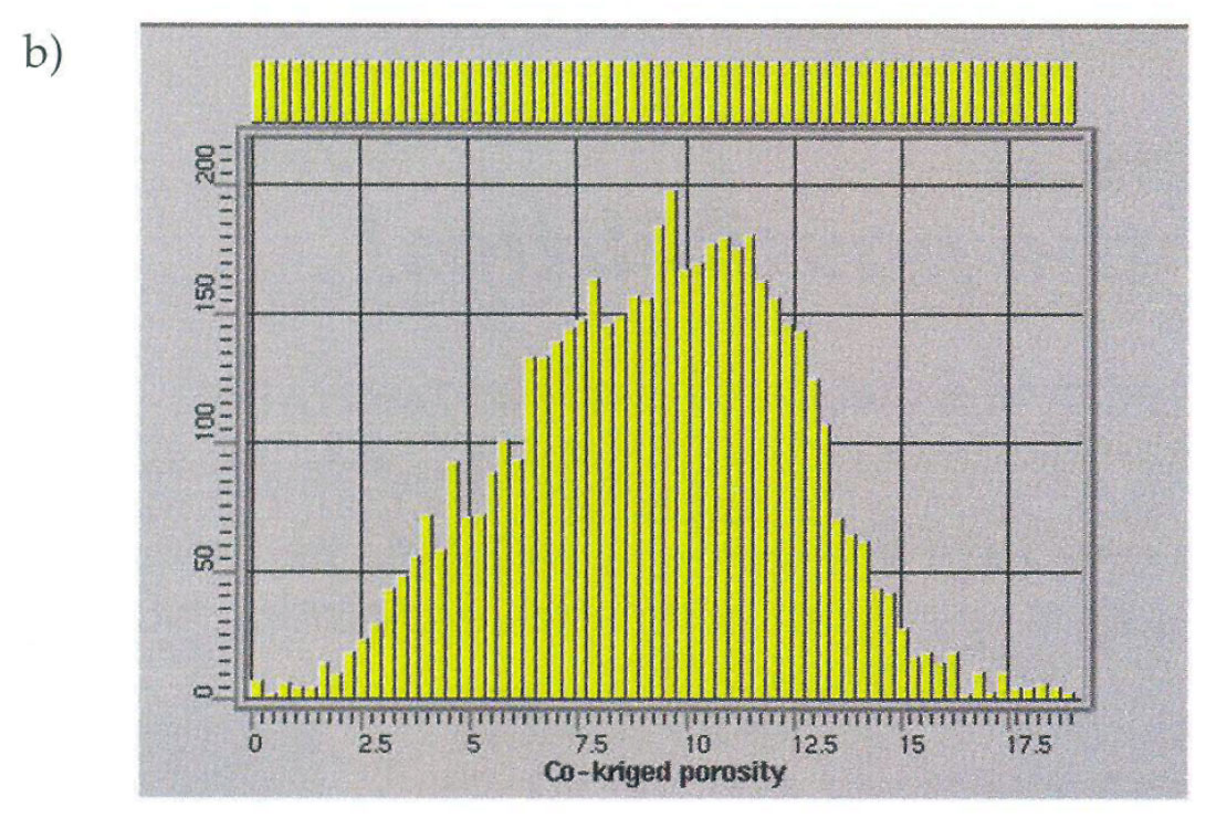
Statistical analysis of the cokriged map can often reveal problems in the final maps that might otherwise go unnoticed. Figure 8a shows a histogram derived from well information in another geostatistical study of a channel sand reservoir area. The two distinct modes in the histogram relate to wells that intersected channel sands and wells that hit the low porosity inter-channel lithologies. A seismic attribute appeared to be correlated with the average porosity at the well locations and was used to guide the interpolation of porosity through collocated cokriging. The histogram of the final porosity map (Fig. 8b) reveals that the bi-modal character of porosity has been lost and the low porosity areas are not well represented in the final maps. This clearly indicates that porosity was non-stationary in this example and the channel and non-channel areas required separation prior to porosity mapping.

Several techniques exist for classifying areas of the field into discrete populations or facies types prior to cokriging. Some of these techniques are based on the well information alone (Indicator Kriging) and other techniques rely on seismic attributes ( discriminant analysis, clustering, etc.). One group of techniques combine information from the wells and seismic attribute data (Sequential Indicator Simulation, Bayesian Sequential Indicator Simulation, etc.) When non-stationarity exists in the reservoir it is very important to perform these classification techniques prior to cokriging based estimation or simulation techniques.

G. Assessing uncertainties in the study

Case study

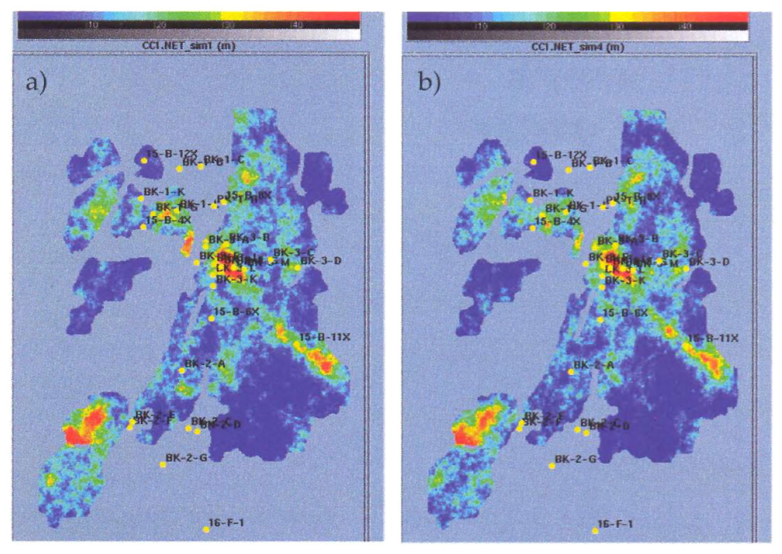
We used a collocated cokriging based Sequential Gaussian Simulation tool, to create a number of maps that were consistent with the available well and seismic information to assess the uncertainty in our mapping of the sand thickness (Figs. 9). There was very little variation among maps, because isochron and sand thickness were so strongly correlated. In our case the largest uncertainties were actually related to the regression relationship between the well and seismic information. We generated several simulations for a number of plausible statistical models to study the effect of the uncertainty of this calibration. Finally, after these uncertaii1ties were considered, there was still an additional source of uncertainty remaining in the model due to the problems in picking the top and bottom of the reservoir in areas of the field that contained crossing channel systems. We noted this additional source of uncertainty in the final report.

General discussion

Once a geostatistical map is generated, it is essential to evaluate its reliability. This can be done using two methods – cross-validation and simulations.

Cross-validation

The analysis of the prediction errors from a cross-validation exercise will give an indication of the mapping uncertainties. Cross-validations should be considered only as one tool in the evaluation of uncertainty. It gives an a posteriori view of the prediction uncertainty and provides an estimate of overall uncertainty that may not be fully representative of the new drilling locations. In particular the uncertainties should be studied spatially, because they vary in space according to the proximity of the wells, the correlogram model used, and the correlation with seismic attributes. For this type of uncertainty analysis, simulations must be run.

Simulations

Simulation techniques generate a family of non-unique maps or volumes that reproduce the variability that is present in the data and modeled by the correlogram. In addition, the processes honor the well information and the correlation with seismic attributes, if they are used. The simulation maps have a more realistic spatial variation than the smooth cokriged map, and each is a possible representation of the reservoir.

Running a number of simulations (at least 50-100) will provide an adequate sample of the possible variation for each point on the map. The prediction uncertainty for a new drilling location, can then be evaluated by producing a histogram of the simulated values at that particular bin location. From the cumulative histogram one can read the prediction uncertainty for a given confidence level.

Sequential Gaussian Simulation requires that the well and seismic data are normally distributed. If the data is not normally distributed, then the variables must be transformed into nom tal score space prior to simulation and the results must be back transformed to the original distribution space.

List of considered uncertainties

The uncertainty estimate should be accompanied by a list of the sources of uncertainty that were considered in the analysis. We often disregard the possibility that basic geostatistical modelling assumptions are not being met. These assumptions include:

1. Petrophysical estimates at the well locations are accurate and error-free.
2. The spatial correlation model is correct
3. Sample statistics from the well data and seismic attributes at the wells are representative of the entire population; etc.

Error in these factors frequently lead to an under-evaluation of uncertainty. An improvement in the overall uncertainty estimate can be achieved by performing simulations and cross-validations using a range of statistical models that fit the available data. The assumptions made in this uncertainty analysis should be recorded in the final report.

Uncertainties in the seismic interpretation and the geologic model are often not considered within the scope of a conventional geostatistical project and this can also result in a poor estimate of the total uncertainty. This uncertainty can be explored to some degree by testing alternate geological scenarios or using a range of seismic interpretations. In any case, the treatment of these uncertainties should at least be mentioned in the report.

IV. Summary and Conclusions

Geostatistical mapping techniques offer a powerful framework for the integration of seismic, geological and petrophysical information into a unified model of the subsurface. Modern, user-friendly software packages, have accelerated the use of geostatistics in the petroleum industry. The responsibility of the geoscientist is to ensure that the results are truly representative of the data and consistent with the geologic model. This includes quality control of the various forms of data, calibrating the well log and seismic information, and creating a reasonable estimate of the uncertainties that are present in the final model.

Well information is always sparse and biased, and seismic information is a non-unique measurement of subsurface properties; therefore, interpretive judgments are an integral part of any geostatistical study. These decisions should be consistent with all available geologic and geophysical information, and they should be fully documented in the final reports. This will allow other geoscientists and engineers to make an informed evaluation of the quality of the study.

As a minimum set, final reports should include the following:

1. Display of a typical well log response
2. Display of a typical seismic section (if seismic information is available and used).
3. Explanation of the seismic attributes that were extracted for use in cokriging
4. Display of the extracted attribute map(s)
5. Base plot showing the location of wells and the reservoir property value at the wells
6. Histogram display of the well log information
7. Histogram display for the correlated seismic attribute (if it is used)
8. Spatial correlation model derived from the well data
9. Spatial correlation model derived from related seismic attributes (if they are used)
10. Cross-plot between tl1e seismic attribute and the reservoir property (if seismic is used) Outlier values should be flagged and discussed Regression relationship should be shown and statistical reliability should be addressed Physical basis for the correlation should be discussed and supported by modelling (where possible)
11. Kriged map with associated error map
12. Cross validation from kriging
13. Reservoir property map based on linear regression (if seismic attributes are used)
14. Cokriged map with associated error map (if seismic attributes are used).
15. Cross validation from cokriging (if seismic attributes are used)
16. Uncertainty estimation based on conditional simulations and cross validation
17. List of considered uncertainties

Suggestions for further reading (by subject):

Calibrating the seismic attribute to the reservoir property:

Boerner, S.T., S. C. Leininger, A. Sunaryo, W. Alexander, J. Gould, M. Sulitra, B. Sabin, and M. W. Do bin, "Analysis, inversion, geostatistical simulation, and visualization of porosity in a carbonate gas reservoir", OTC 8288, presented at the 1997 Offshore Technology Conference held in Houston, TX, 5-8 May, 1997.

Hirsche, K., Porter-Hirsche J., Mewhort L., Davis R., "The Use and Abuse of Geostatistics", The Leading Edge, March, 1997, pp. 253-260.

Kalkomey, C.T., Potential risks when using seismic attributes as predictors of reservoir properties, The Leading Edge, March, 1997, pp. 247-251.

Matteucci, G., "Seismic attribute analysis and calibration: a general procedure and a case study." Exp. Abs. 66th Annual SEG meeting (Denver) 1996.

Mapping with non-linear relationships between seismic attributes and reservoir properties:

Castaldi, C., Doyen, P., Roy, D., and den Boer, L., "Seismic Thickness Prediction under Tuning Conditions by Bayesian Simulation", The Leading Edge, March 1998.

Classification of data on the basis of lithology:

Doyen, P.M., Psaila, D.E., and Strandenes,R.M., "Bayesian sequential indicator simulation of channel sands from 3-D seismic data in the Oseberg field, Norwegian North Sea", SPE 28382, 69th Ann. Tech. Confr. and Exhb., SPE.

Geostatistical case history:

Castaldi, C., Biguenet, J.P., Pazzis, L., "Reservoir Characterization from Seismic Attributes: An example from the Peciko Field (Indonesia)", The Leading Edge, March, 1997, pp. 263-266

General introductions to geostatistics and cokriging:

Isaaks, E. H. and Srivastava, R. M., An Introduction to Applied Geostatistics, Oxford University Press, 1989.

Doyen, P.M., "Porosity from Seismic Data – a Geostatistical Approach", Geophysics, 1988