Automatic high-density constrained velocity picking

Introduction

Velocity analysis is one of the main steps in seismic processing. A velocity model, beyond its initial purpose to obtain a seismic stack, is used for time and depth imaging, AVO analysis and inversion, pore pressure prediction and so on. In conventional processing, it is a high cost procedure and it requires a great deal of manual work. In this paper I present a method for high-density automatic velocity analysis.

Semblance-based coherency measures are commonly applied to perform velocity analysis (Taner and Koehler, 1969) on seismic reflection data. Velocities are estimated by maximizing a coherence measure with respect to the hyperbolic parameter. The main idea is that we look for stacking velocities for each CDP gather and a dense set of the time samples using the threshold for the semblance. The program finds all constrained values of stacking velocities where possible (where the semblance value is larger than the threshold). To find the constraints for the stacking velocities, one may pick a velocity manually at several points and determine the constraints. Then we take these CDP gathers as the reference points and extend picked velocities for the whole line area.

Stacking velocities

The velocity field is one of the most important factors in seismic processing. Accurate knowledge of seismic velocities is essential for transforming surface reflection time data into depth images of reflector locations. We should distinguish two kinds of velocity. From real data we directly extract velocities in the time domain, which give us the best image (stack). We can call these stacking velocities or time-imaging velocities. If we want to obtain a depth image through depth migration or simply to perform a time-to-depth transformation, we have to use a depth velocity model. In this paper we will consider only stacking velocities. The conventional approach assumes manual velocity picking for several CDP gathers and subsequent interpolation for the line for 2-D data, or for the volume for 3-D data. For many procedures, such as time migration, or AVO analysis or even when the stacking velocities change rapidly, we need an accurate velocity field. Fast lateral fluctuations of stacking velocity may be caused by shallow velocity anomalies even in the subsurface with gentle dipping boundaries (Blias, 2005). In this case we also have the issue of reliability of stacking velocities related to the density of sampling. At the same time, velocity can be quite damaging if we get it wrong and it can also be very time consuming to determine it properly.

In addition to obtaining correct estimates of the velocity, we also have the question of its reliability related to the sampling density. From geological constraints, and since CDP gathers are highly overlapped, we know that velocity cannot change rapidly within adjacent CDP gathers. This implies that to describe adequately lateral and vertical stacking velocity changes we can use a much smaller number of parameters then the input data. On the other hand, we know that we cannot expect to determine a reliable stacking velocity for each time sample of the CDP gather. This is because for the coherence based approach (the same as any other) our assumptions are not satisfied for most time samples. The main assumption in any automated velocity picking is that there is only one wave within the considered time window.

Let’s briefly consider the restrictions on applying a locally 1-D model to velocity analysis. Strictly speaking, RMS velocity and Dix’s formula have been derived for infinitely small spreadlength for a 1-D layered velocity model, that is for the model with horizontal homogeneous boundaries. That is why one often reads that conventional velocity analysis is based on a layered media assumption. In reality we never have horizontal boundaries and homogeneous layers and if we had this subsurface, we would not need seismic exploration! For this kind of subsurface it’s enough to know the velocity distribution at one point. Fortunately, we can use Dix’s formula in many real situations even when there are lateral changes in the subsurface velocities, as well as when we have a long spreadlength.

The important practical question is: How far can we go from this assumption? In other words, when can we assume that stacking velocities are close to RMS? Dix’s formula gives a reasonable estimation of interval velocity when and only when stacking velocities are close to RMS. At first glance the answer would be that we can use Dix’s formula when the subsurface is close to a 1-D model; that is the medium has almost horizontal boundaries with almost homogeneous layers. But this is not strictly right because we have seen cases with significant dip when Dix’s formula gives reasonable interval velocity estimations and we can see that sometimes even relatively small lateral velocity changes cause large deviations of stacking velocities from RMS, and, therefore, from average velocities.

It was analytically shown and illustrated with modeling (Blias, 1981, 1988, 2005a, 2005b) that deviation between stacking and RMS velocity depends on where lateral velocity changes occur. The main reason for the stacking velocity anomalous behaviour (for large deviations from average velocity) is non-linear lateral variations of the overburden interval velocities or their boundaries. The dipping boundaries and linear changes in interval velocities (boundary and velocity gradients) do not cause large changes in the stacking velocities. They don’t prevent the use of the Dix formula to find interval velocities.

Important note about stacking and RMS velocities

Sometimes geophysicists call stacking velocities RMS. We should mention that even for the subsurface with horizontal homogeneous layers stacking velocity, as obtained from any velocity analysis, is never equal to RMS velocity, even in theory. To explain this, let’s consider the NMO function t(x). We can expand it into a Taylor series (Taner and Koehler, 1969):

Here t₀ is zero-offset time, VRMS is a parameter, defined by the formula:

Here If we truncate the series to the second power of x then

This is a hyperbolic equation. Coefficients c₂, c₄, ... are small but they equal 0 only for homogeneous medium. This means that for any non-homogeneous subsurface, stacking velocity differs from RMS velocity and only for the homogeneous velocity model does V_Stack ≈ V_RMS. Usually coefficients c₂, c₄, … are small, we can neglect them and that is why V_Stack = V_RMS. The main difference between RMS and stacking velocities is that they represent two different notions. RMS velocity is a velocity defined by a mathematical relation (V_RMS) and stacking velocity is a velocity found from the hyperbolic approximation of a non-hyperbolic NMO curve t(x). In many cases they are close but nevertheless, it’s better not to mix these two notions.

Automated velocity picking. We can now ask ourselves several important questions. First of all, do we need an automatic high-density velocity picker? We already know the answer to this question: we need it in situations with lateral changes of stacking velocities; we need it for the large 3-D data sets to save time in velocity picking; we need it to improve velocity models for AVO; and we need it for better seismic imaging quality. The second question might be: Can we trust the results of automatic velocity picking? This question has an easy answer: we have several QC controls, namely NMO gathers (flat reflections), better imaging quality, and more reasonable depth velocity models, which are all determined from NMO curves.

We use a coherence measure to estimate the NMO function. The main problems with this approach are:

(i) Non-uniqueness. Which arises because of coherence semblances. Often there are more than one local maxima for the one zero-offset time value, mostly caused by mulpiples. To solve this problem, we use constraints, which allow us to separate primaries from multiples. To calculate areal constraints, we create supergathers at several points of the area, usually from 10 to 100 reference points, depending on the local geology. At these points, we stack thousands of traces to create supergathers, which demonstrate velocity properties around the reference point. Usually the subarea covered by the supergather is about 2 – 4 km2. For each supergather we pick stacking velocities and this manual or automatic picking is a relatively easy one. Then the program analyzes these velocities and calculates constraints for the high-density automatic velocity analysis.

(ii) High-frequency velocity oscillations. To remove these kind of deviations, we use median smoothing.

(iii) Non-hyperbolic NMO curves. To pick non-hyperbolic NMOs, we use additional parameters to describe the NMO curve τ(x):

where x_k is an offset for the k-th trace in the CDP gather, V_Stk is a stacking velocity, α are unknown parameters to be calculated, fj(k), j = 1, 2, …, J; J stands for the number of even basis functions fj; usually, j = 1 or 2.

(iv) Class II AVO response. Semblance velocity analysis is based on the assumption of constant amplitude and does not take into account amplitude variations with offset. It becomes an important problem when the amplitudes change their sign (Class II AVO response, Rutherford and Williams, 1989). To take into account AVO effects, we can use a method similar to the approach suggested by Sarkar et al. (2001). We can consider the generalization of the semlance method to include AVO effects:

where U_i(t) is a seismic trace at the offset x_i, τ_I(v) is an NMO function, A(t) and B(t) are AVO parameters; t₀ is the zero offset time for which we find the stacking velocity V_Stk(t₀). Parameters A and B can be found from the system of equations:

It can be shown that if we consider B(t) = 0, then (1) is the same as conventional coherence measure, introduces by Taner and Koehler (1969):

It can be shown that if we cons

Model testing. Let’s analyze the stability and uncertainty of AVO velocity analysis on model data with a Class II AVO response. Figure 1 shows synthetic gathers with primaries, multiples and different noise levels.

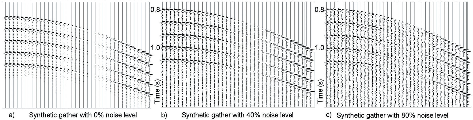
Figure 2 displays generalized and conventional coherence measures generalized for the different noise levels. From the model the value of the stacking velocity should be 2.4 km/s. These pictures show that taking into account the AVO effect in the coherence measure gives more accurate velocity values when we have reversed polarity amplitudes. Figure 2 shows the coherence measure, calculated from formula (1) (left) and (2) (right). Figure 2a corresponds to the synthetic gather with 0% noise level. This gather is plotted on Figure 1a. Figure 2b displays the coherence measure for the gather on figure 1b and figure 2c corresponds to the gather shown on figure 1c.

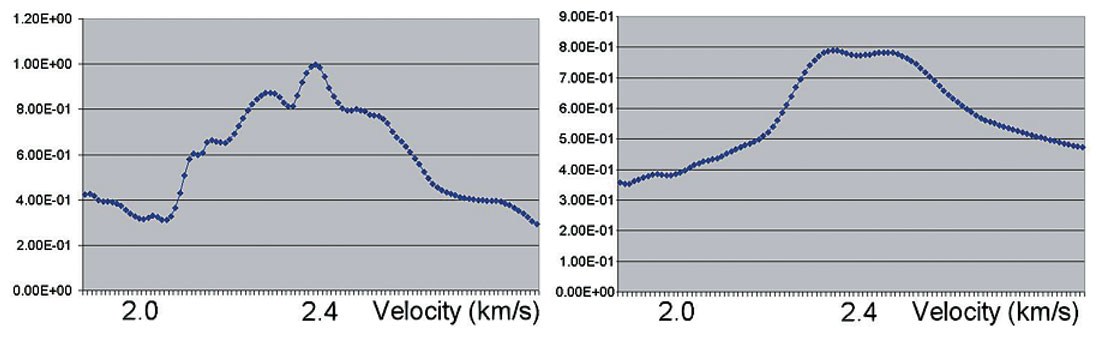
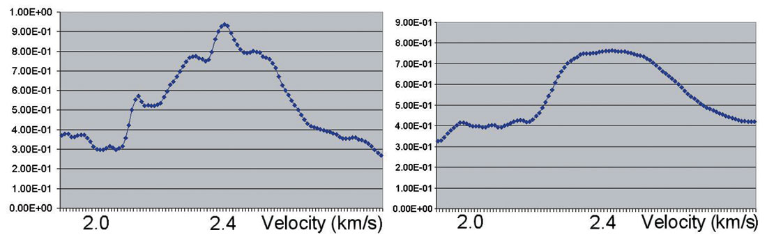
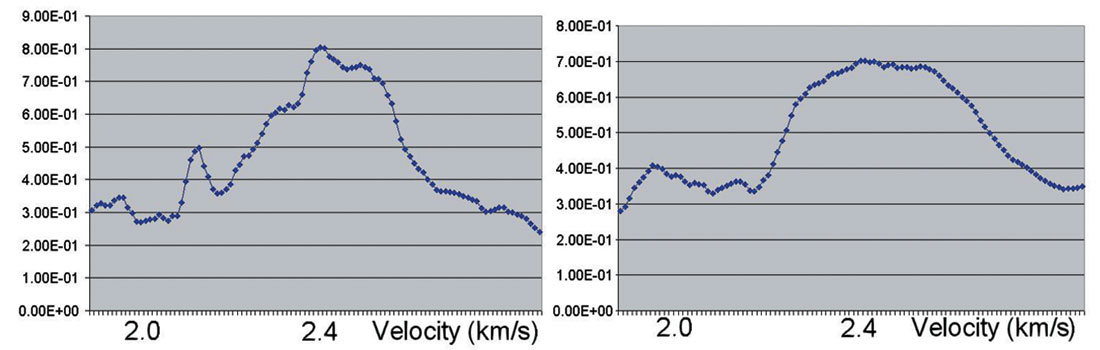
From these examples we come to the conclusion that for a class II AVO response the generalized semblance has much less uncertainty than the conventional one for any noise level.

Interval velocity analysis. Conventional velocity analysis works in two steps:

(i) We scan CDP gathers with a coherency measure (velocity spectrum or semblance) using hyperbolas. These hyperbolas are parameterized with two parameters: zero-offset time T₀ and a stacking velocity V_S. We measure the semblance for a set of hyperbolas and transform the CDP gather traces from the offset and time coordinates into the coherence semblances in coordinates of time and stacking velocities.

(ii) We then pick local maxima of these coherence semblances and assign zero-offset time and corresponding stacking velocities.

This method, presented by Toldi (1989), assumes that we can use RMS velocity as a reasonable estimation of stacking velocity. Then we can scan the CDP gathers not for the stacking, but for the interval velocity and calculate RMS velocity for each value of the interval velocity. As was shown by Blias (1981, 2005a, 2005b) in the case of the subsurface having modest dipping boundaries and moderate deep interval velocity changes, we can consider the RMS velocity as close to the stacking velocity and use this approach. In the presence of not properly accounted for shallow or overburden velocity anomalies, the difference between stacking and interval velocities can be quite large (up to 30% and more). Therefore before using this approach we have to remove the effects of the lateral velocity changes in the overburden.

Automated Velocity analysis in the presence of shallow velocity anomalies. Shallow velocity anomalies cause fast lateral variations in the stacking velocity, increasing with depth. As was shown by Blias (2003), application of a generalization of Dix’s formula to a laterally inhomogeneous layer gives a reasonable estimation of the interval velocity. We can then include analytical traveltime inversion into automated velocity analysis. For this the program automatically picks the velocity for the shallowest horizon, determines interval velocity in the first layer and then predicts the stacking velocities, using formulas developed by Blias (1981, 1988, 2005 a, b). Then the automated velocity picker simply determines stacking velocities in a layer-stripping manner around predicted values.

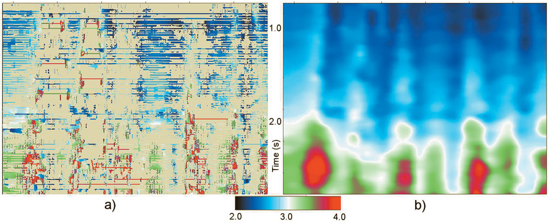
As was mentioned in the introduction, the main concept behind an automated high-density velocity analysis is quite clear – we pick velocities for all of the time samples and all the CDP gathers where the coherence measure exceeds the threshold value. Since coherence measure is normalized within the range from 0 to 1, we use for the threshold a value from 0.2 to 0.5 depending on the data quality. After picking high-density velocities, we fill the gaps and smooth the velocity field using geologically consistent constraints. Figure 3 shows the map of automatically picked stacking velocities (a) and after filling gaps and smoothing (b).

Lateral variations in the stacking velocity field, increasing with depth, clearly indicate the presence of shallow velocity anomalies (Blias 1988, 2005a, 2005b).

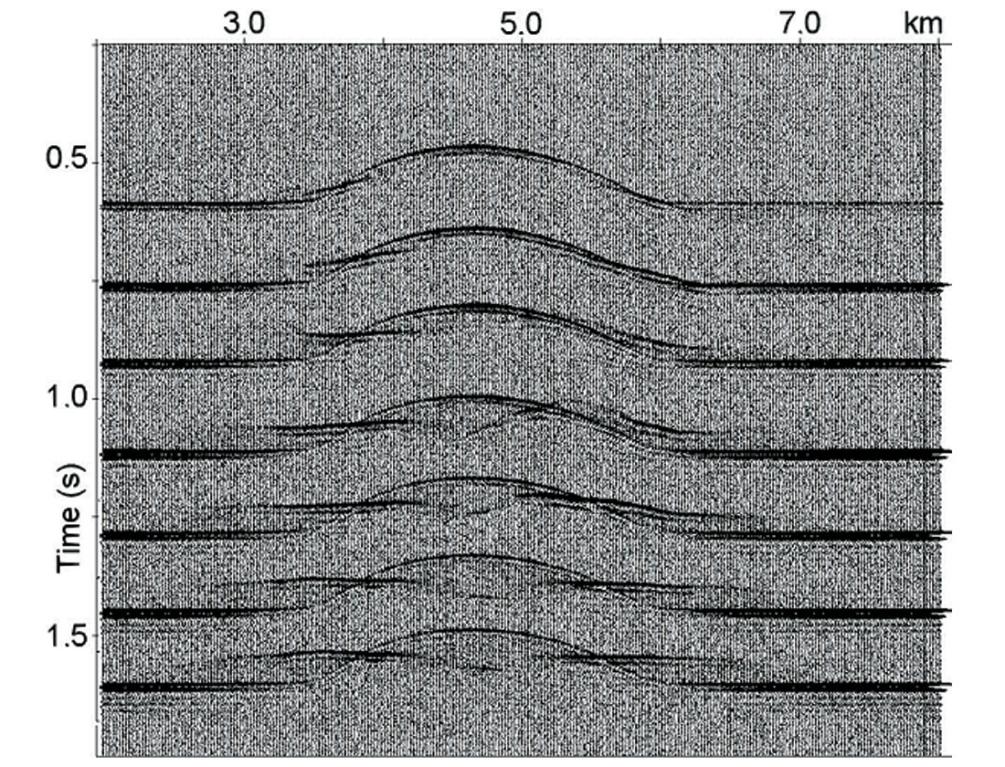
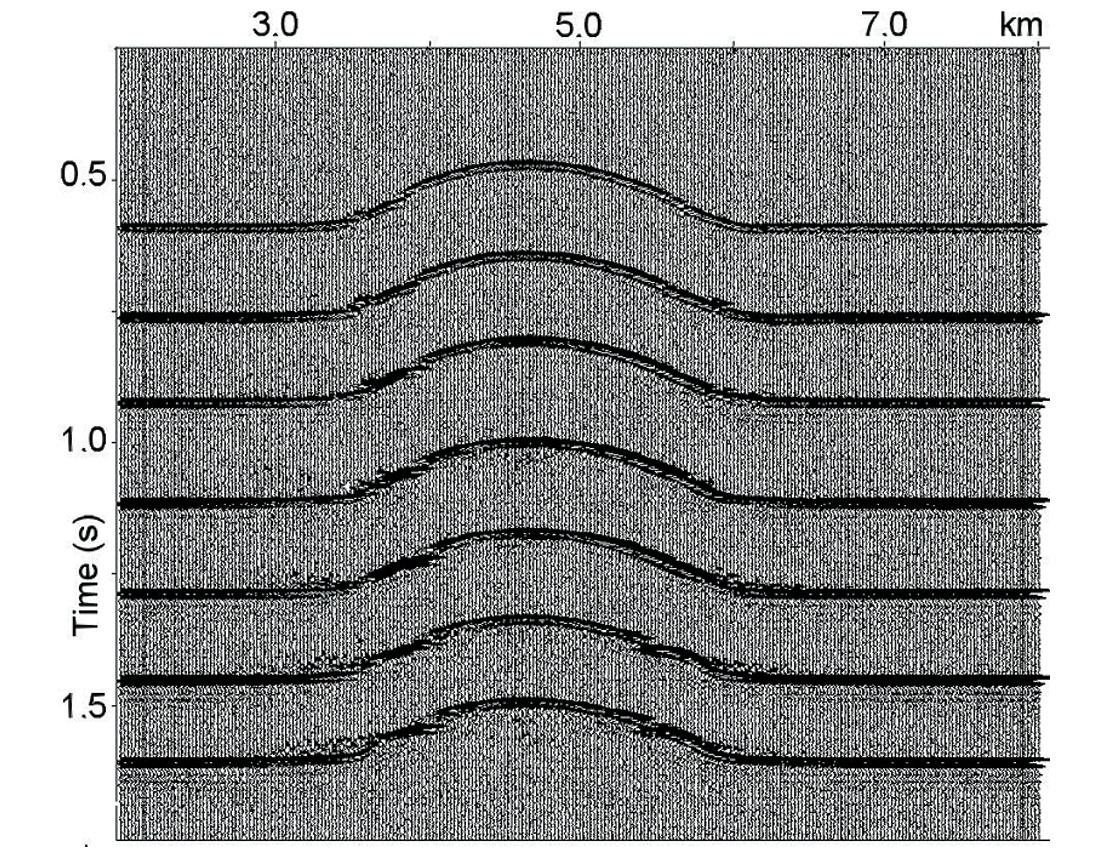
Model data example. To test automated high-density velocity analysis for data with fast lateral changes in the stacking velocity field and non-hyperbolic NMO curves, we created a depth velocity model (Figure 4). All boundaries except the bottom of the first layer and all interval velocities except the first one are constant. A shallow velocity anomaly is created by a curvilinear boundary and allowing the first layer interval velocity to increase from 1.6 km/s to 2.5 km/s. For this model synthetic CDP gathers have been created with maximum offset / reflector depth ratio of 1.25. The shot interval is set equal to the receiver interval at 20 m. Random noise has also been added to the gathers. These CDP gathers are displayed on figure 5. Figure 6 shows the velocity field after automatic continuous velocity analysis. We see large lateral stacking velocity oscillations increasing with depth.

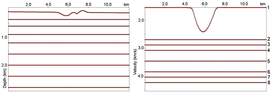
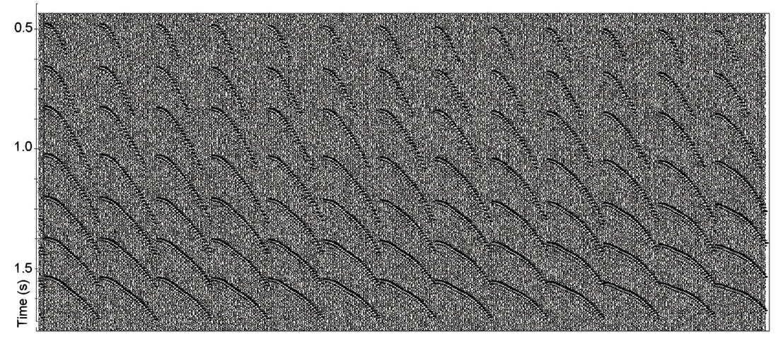
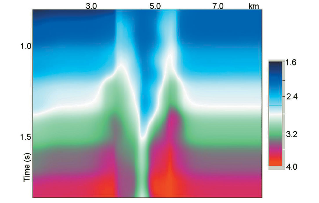
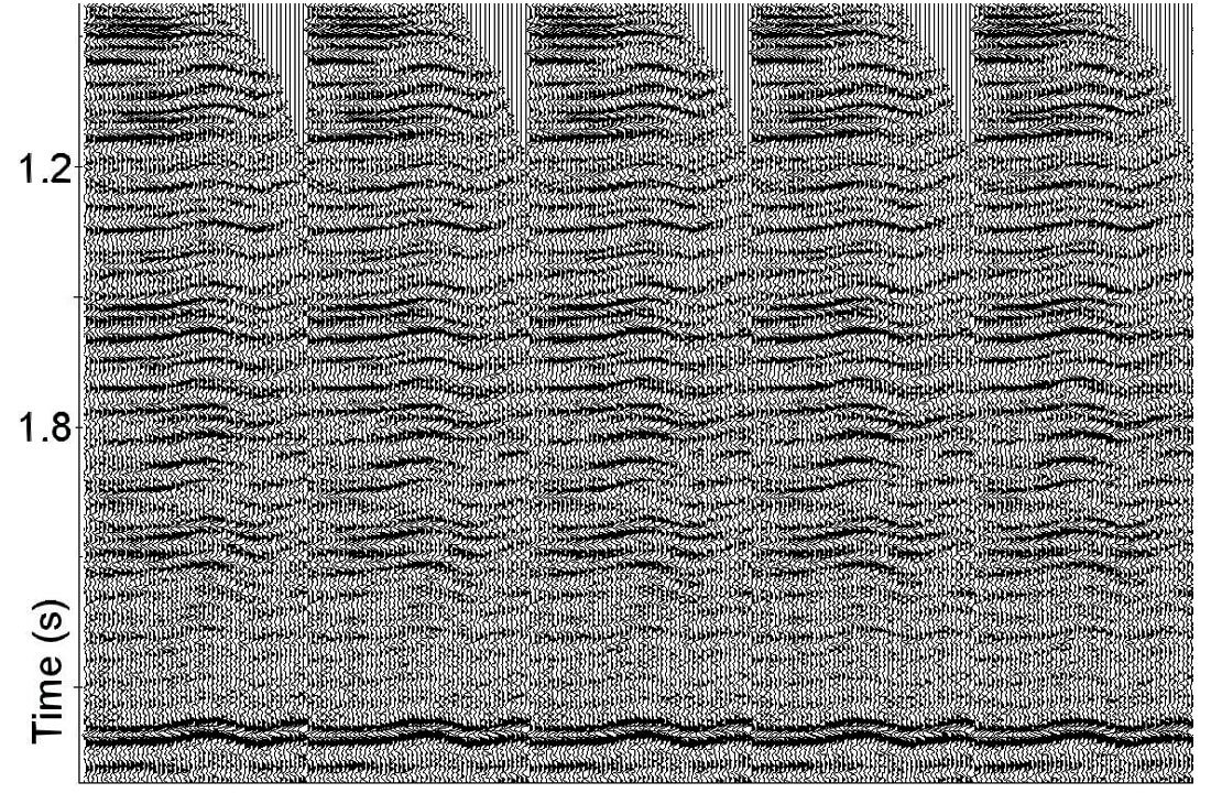
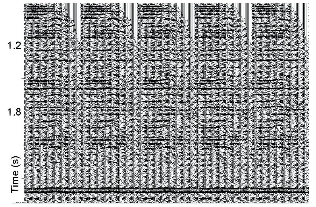
Figure 7 shows CDP gathers after hyperbolic (a) and non-hyperbolic (b) automatic high-density velocity analysis close to the center of velocity anomaly. We see that for this model NMO curves differ significantly from hyperbolas.

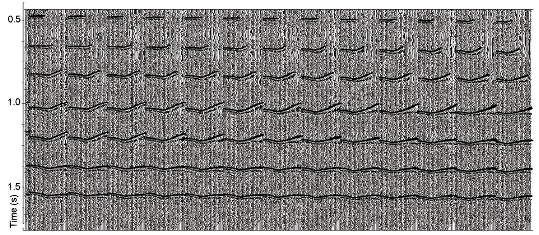
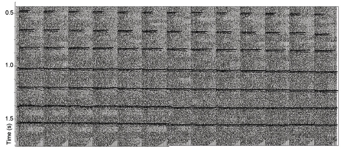
Figure 8 displays post-stack data obtained from hyperbolic (a) and non-hyperbolic (b) NMO gathers. We see that non-hyperbolic NMO significantly improves the post-stack image within the intervals around the shallow velocity anomaly. Here we should mention that shallow velocity anomalies may not cause non-hyperbolic NMO but they always cause significant lateral variation of the stacking velocity at deep reflectors (Blias, 2005a, 2005b).

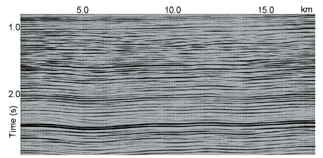
Real data examples. Let’s first consider a seismic line with shallow velocity anomalies. A non-first-break approach of determination and removal of the effects of these anomalies (Blias, 2005) needs horizon-based stacking velocity information. Figure 9 shows CDP gathers after automated high-density velocity analysis: hyperbolic NMO (a) and non-hyperbolic NMO (b).

Shallow velocity anomalies are often the origin of non-hyperbolic NMO curves as well as of lateral variations in the stacking velocity field, the effect increasing with depth (Fig. 10a), and general poor imaging quality. To determine and remove the effects of shallow velocity anomalies, we applied a non-firstbreak approach (Blias, 2005 a, b). In this method, we use the results of horizon-based high-density automated velocity analysis to build a depth velocity model. We then use the depth velocity model to remove the influence of the shallow velocity anomalies. For this we run a raytracing for the obtained depth velocity model and calculate pre-stack reflection time arrivals for all boundaries.

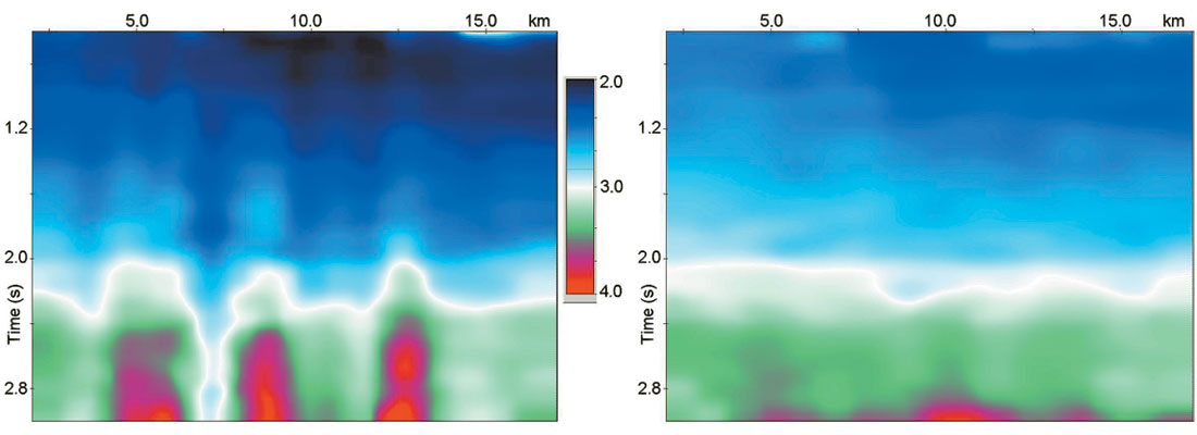
Subsequently we replace the shallow inhomogeneous layer with a homogeneous one and calculate time arrivals for this model. The difference between the first and the second set of these times is applied to the CDP gathers. This procedure moves events on pre-stack data to the position where they would be if the shallow layer were homogeneous. Stacking velocities after VR are shown in figure 10b. We see much less lateral fluctuation in the stacking velocity as compared to the initial velocity field (Fig. 10a). Figure 11 shows post-stack data before (a) and after (b) the shallow velocity replacement. We can see that VR significantly improved the post-stack image quality as well as the velocity field.

Marine data. Let’s consider an example of automatic high-density velocity analysis on marine data with a high noise level. Figure 12 shows the initial CDP gathers (a), the same gathers after hyperbolic NMO (b) and non-hyperbolic NMO (c). Figure 13 displays a supergather, calculated from 16,000 traces to pick initial velocities and generate the constraints for the automatic high-density velocity analysis.

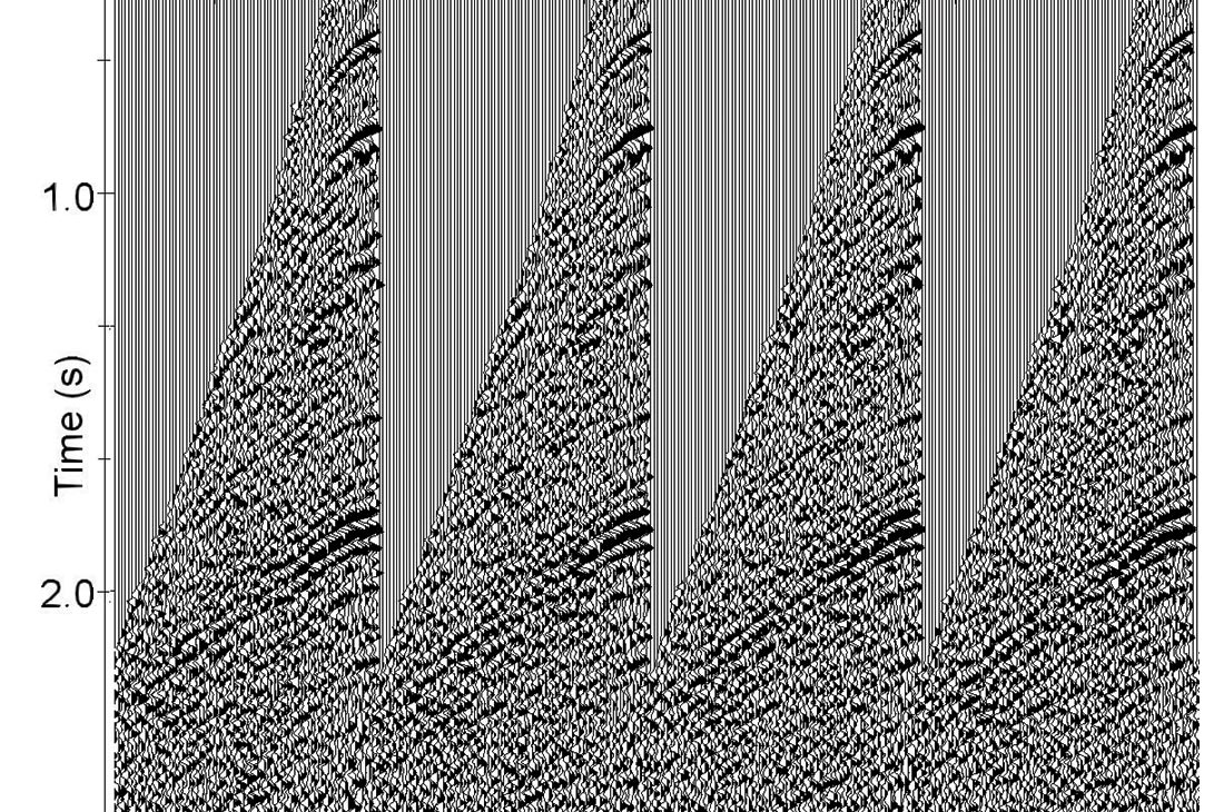
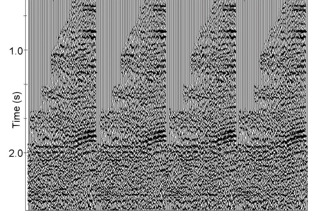
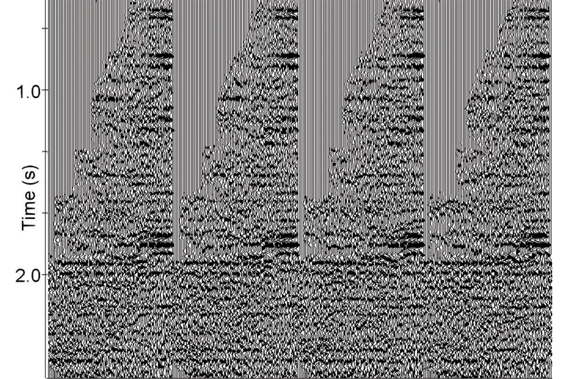
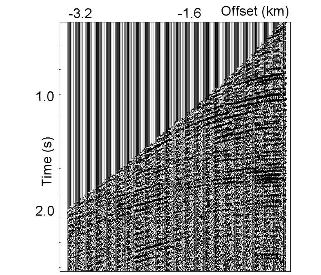
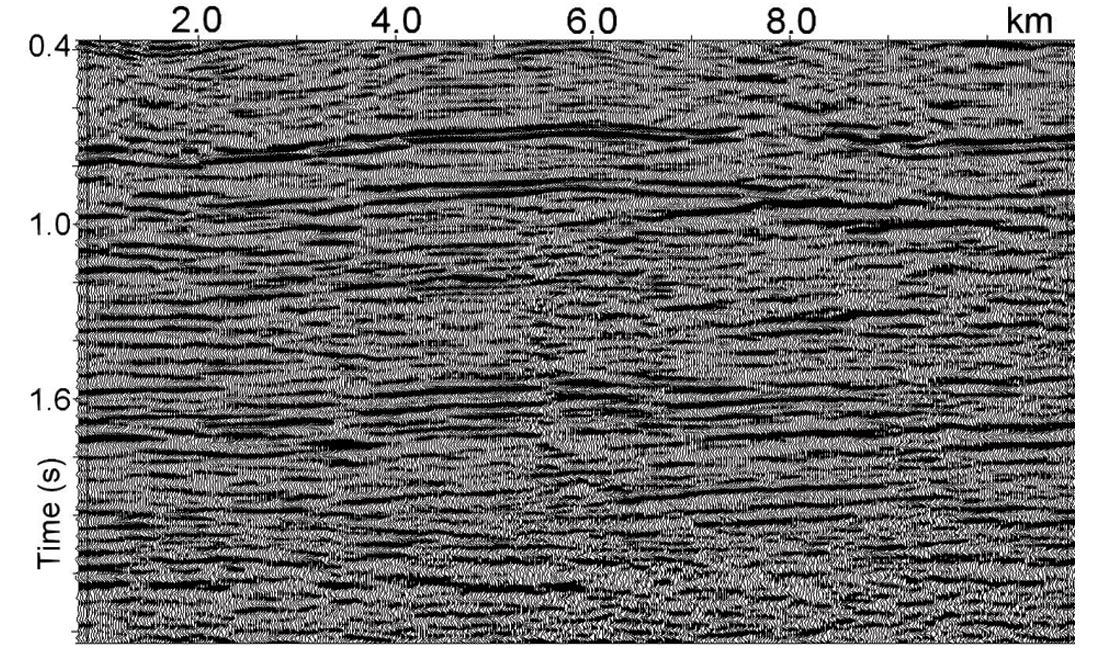
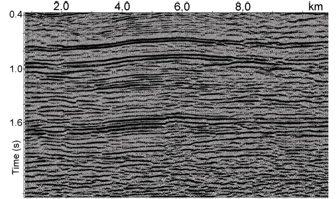
Figure 14a shows the stacked section after the application of conventional velocity analysis (500 m interval manual picking). We see the effects of fast lateral velocity changes caused by overburden velocity anomalies. Here we should reiterate that manual velocity picking is an expensive task, both in terms of time and cost. It also might be important to have a dense velocity field to reduce velocity interpolation errors between the analysis locations. We already know that shallow velocity anomalies lead to fast lateral velocity changes. This implies the need for high density velocity picking for better stack response and for recovering the shallow velocity anomalies when the first break technique does not work. Sometimes a conventional velocity analysis (manual velocity picking with the interval of 500-1000 m and interpolation) might leave residual errors in the stacking velocities. Figure 14b displays the stacked data after automatic high-density velocity analysis. Comparing figure 14a and 14b we see that automatic high-density velocity analysis leads to a more accurate velocity field and, consequently, to more consistent events on the poststack data.d, consequently, to more consistent events on the poststack data.

Conclusions

For some problems (time migration, depth velocity model building, AVO, pore pressure prediction) we need high-density reliable stacking velocities at each CDP gather. To utilize the advantage of high-density automatic velocity analysis, we have to determine and use geologically consistent constraints. Several generalizations for automatic velocity analysis have been developed for different cases. They take into account fast lateral velocity changes and AVO effects. An automatic high-density velocity picker can be applied to pre-stack data with different quality. It allows us to obtain reliable stacking velocities even with non-hyperbolic NMO curves. NMO functions can then be used to build a depth velocity model for pre-stack and post-stack depth migration.

Acknowledgements

I would like to thank Michael Burianyk (Shell Canada) for his assistance in preparing this paper. I would also like to acknowledge Valentina Khatchatrian who developed most of the velocity analysis software and Samvel Khatchatrian for useful discussion.