Application of texture attribute analysis to 3D seismic data

In this study, texture attribute analysis application to 3D surface seismic data is presented. This is done by choosing a cubic texel from the seismic data to generate a grey-level occurrence matrix, which in turn is used to compute second-order statistical measures of textural characteristics. The cubic texel is then successively made to glide through the 3D seismic volume to transform it to a plurality of texture attributes. Application of texture attributes to two case studies from Alberta confirm that these attributes enhance understanding of the reservoir by providing a clearer picture of the distribution, volume and connectivity of the hydrocarbon bearing facies in the reservoir.

Introduction

A plethora of seismic attributes have been derived from seismic amplitudes to facilitate the interpretation of geologic structure, stratigraphy and rock/ pore fluid properties. Complex trace analysis (Taner and Sheriff, 1977) treats seismic amplitudes as analytic signals and extracts various attributes to aid feature identification and interpretation. Computations for these attributes are carried out at each sample of the seismic trace and so have also been dubbed instantaneous attributes. Another class of attributes utilizes the 3D nature of the seismic data by using an ensemble of traces in the inline and crossline directions and using time samples in the computation as well. Coherence attribute computation is done this way. More information on all these attributes can be found in Chopra and Marfurt, 2005. These different attributes have been used for different purposes and have their own limitations.

Texture analysis of seismic data was first introduced by Love and Simaan (1984) to extract patterns of common seismic signal character. This inspiration came from the suggestion that zones of common signal character are related to the geologic environment in which their constituents were deposited. These and other similar attempts enjoyed limited success as the outcome was dependent on the signal-to-noise ratio and also because the stratigraphic patterns could not be standardized. More recently, the use of statistical measures to classify seismic textures using grey-level co-occurrence matrices (GLCMs) (West et al, 2002, Gao, 2003) has been introduced.

The idea behind texture analysis of surface seismic data is to mathematically describe the distribution of pixel values (amplitude) in a sub-region of the data. Texture analysis has been extensively used in image processing (remote sensing), where individual pixel (picture element) values are used in the analysis. The term texel (texture element) is usually used for reference to the smallest set of pixels (planar for 2D) used for characterizing a texture. For 3D seismic data, a cubic texel is used for texture analysis. The technique used to quantify this utilizes a transformation that generates GLCMs. The GLCMs essentially represent the joint probability of occurrence of grey-levels for pixels with a given spatial relationship in a defined region. The GLCMs are then used to generate statistical measures of properties like coarseness, contrast and homogeneity of seismic textures, which are useful in the interpretation of oil and gas anomalies.

GLCMs for seismic data

A computed grey-level co-occurrence matrix has dimensions n x n, where n is the number of grey levels. For application to seismic data, the grey levels refer to the dynamic range of the data. For example, 8 bit data will have 256 grey levels. A GLCM computed for this data would have 256 rows and 256 columns (65,536 elements). Similarly, 16-bit data would have a matrix of size 65,536 x 65,536 = 429,496,720 elements, which could be a little overwhelming even for a computer. Usually, the seismic data is rescaled to 4 bit (16 x 16 matrix) or 5-bit (32 x 32 matrix) and in practice it has been found that this does not result in any significant differences in the computed properties.

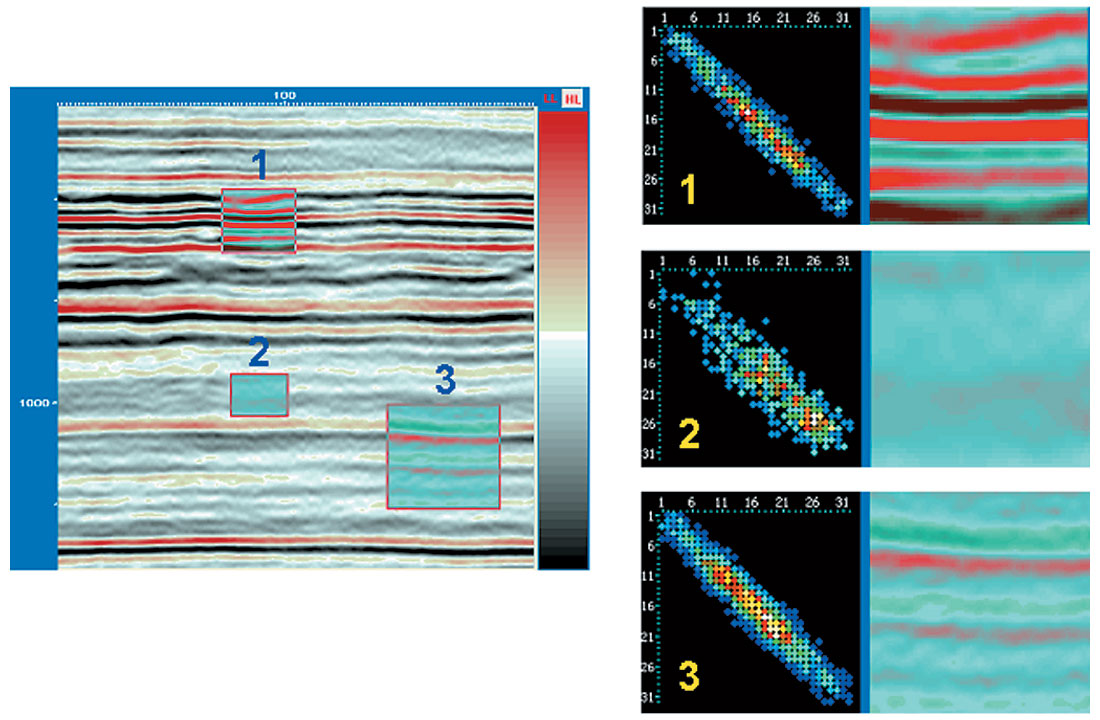
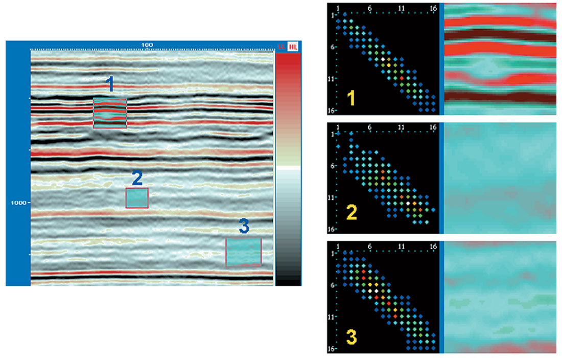
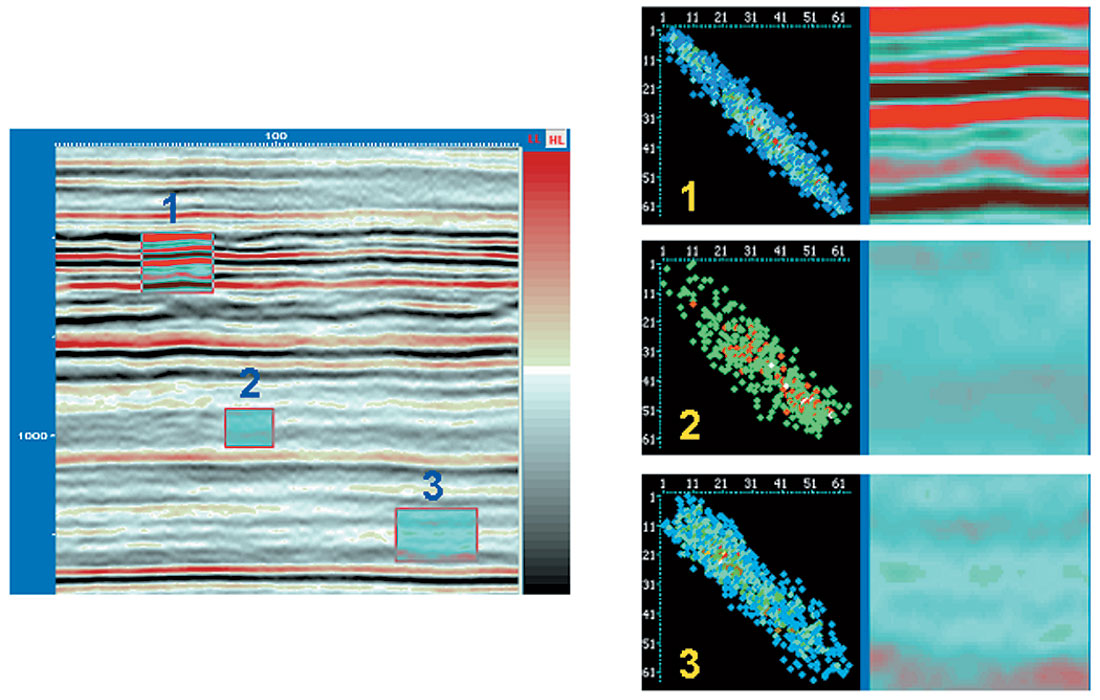
The structure of GLCMs as applied to seismic data can be easily understood. Figure 1 shows the region segments 1, 2 and 3 selected for GLCM computation and the computed GLCMs are shown to the right. For strong continuous reflections, the GLCM exhibits a tight distribution along the diagonal. The matrix size chosen is 32 and the parameters chosen are 4, 3 and 4 in the inline, crossline and time directions. Low amplitude regions exhibit values near the center. Discontinuous or incoherent reflections have more occurrences farther away from the diagonal (view 3 in fig 1). View 2 has lower amplitudes as well as incoherent reflections and so the GLCM shows a scatter about the diagonal. For a matrix size 16, we see smaller number of elements in the GLCM (Figure 2) and for a matrix size 64, there is a higher population of points (Figure 3).

While GLCMs give us all this information, they are not accurate enough to make quantitative interpretations. They need to be matched by extracting a number characteristic property of each matrix. In other words, texture features can be generated by applying statistics to co-occurrence probabilities. These statistics identify some structural aspects of the arrangement of probabilities within a matrix indexed on i and j, which in turn reflects some characteristic of the texture. There are various types of statistics that can be used. Haralick et al (1973) demonstrated the derivation of 14 different measures of textural features from GLCMs. Each of these features represents certain image properties as coarseness, contrast or texture complexity. However, due to redundancy in these statistics, the following four measures generate the desired discrimination without any redundancy.

1. Energy
2. Entropy
3. Contrast
4. Homogeneity

1. Energy: is a measure of textural uniformity in an image. Mathematically, it is given as

Energy is low when all elements in the GLCM are equal and is useful for highlighting geometry and continuity.

2. Entropy: is a measure of disorder or complexity of the image.

Entropy is large for images that are texturally not uniform. In such a case, many GLCM elements have low values.

3. Contrast: is a measure of the image contrast or the amount of local variation present in an image.

Contrast or inertia is high for contrasted pixels while its homogeneity will be low. When used together, both inertia and homogeneity provide discriminating information.

4. Homogeneity: is a measure of the overall smoothness of an image.

Homogeneity measures similarity of pixels and is high for GLCMs with elements localized near the diagonal. Thus homogeneity is useful for quantifying reflection continuity.

For 3D seismic volumes, computing GLCM texture attributes at one location yields the localized features at that point. Repeating the computation of these attributes in a sequential manner throughout the volume, transforms the input seismic volume into the above four texture attributes, which we discuss below.

High amplitude continuous reflections generally associated with marine shale deposits have relatively low energy, high contrast and low entropy. Low amplitude discontinuous reflections generally associated with massive sand or turbidite deposits have high energy, low contrast and high homogeneity (Gao, 2003). Low frequency, high amplitude anomalies generally indicative of hydrocarbon accumulation typically exhibit high energy, low contrast and low entropy relative to non-hydrocarbon sediments.

Application of texture attribute analysis

Sometimes the gas bearing formations are not characterized by very high amplitude bright spots on the prestack migrated seismic data, that any drilling may be risked. Besides, seismic reflection amplitudes are influenced by other parameters such as thickness, lithology, porosity and fluid content and so even if bright spots were present, they would be ambiguous. To resolve such ambiguities we use texture attributes and these provide a detailed and accurate estimates of distribution of reservoir sands in the zone of interest. In the two cases under study here, based on the log correlation, the amplitudes corresponding to sands were somewhat pronounced as seen in the figure, but not conspicuous enough to be picked up as representing anomalies.

Case Study 1

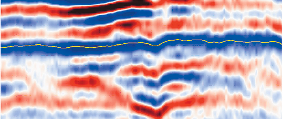
This study focuses on an area in southern Alberta. The target zone is Lower Cretaceous glauconite filled fluvial deposits that have been productive in the area. A 3D seismic survey was acquired in order to create a stratigraphic model consistent with the available well control and matching the production history. The ultimate goal was to locate the undeveloped potential within the fluvial deposits in terms of new drilling locations that could be decided based on the present analysis. As the objective was stratigraphic in nature, the seismic data was processed with the objective of preserving relative amplitudes. Prestack time migration improves our ability to resolve stratigraphic objectives and extract high-quality seismic attributes and so was run on the data. It resulted in an improvement in the stack image in terms of frequency and crisper definition of features as it contributes to energy focusing and improved image positioning prior to stack (Reilly, 2002). Figure 4 shows a segment of a seismic section indicating the reservoir level and the producing sandstone (seen as dark blue) as enclosed in the box.

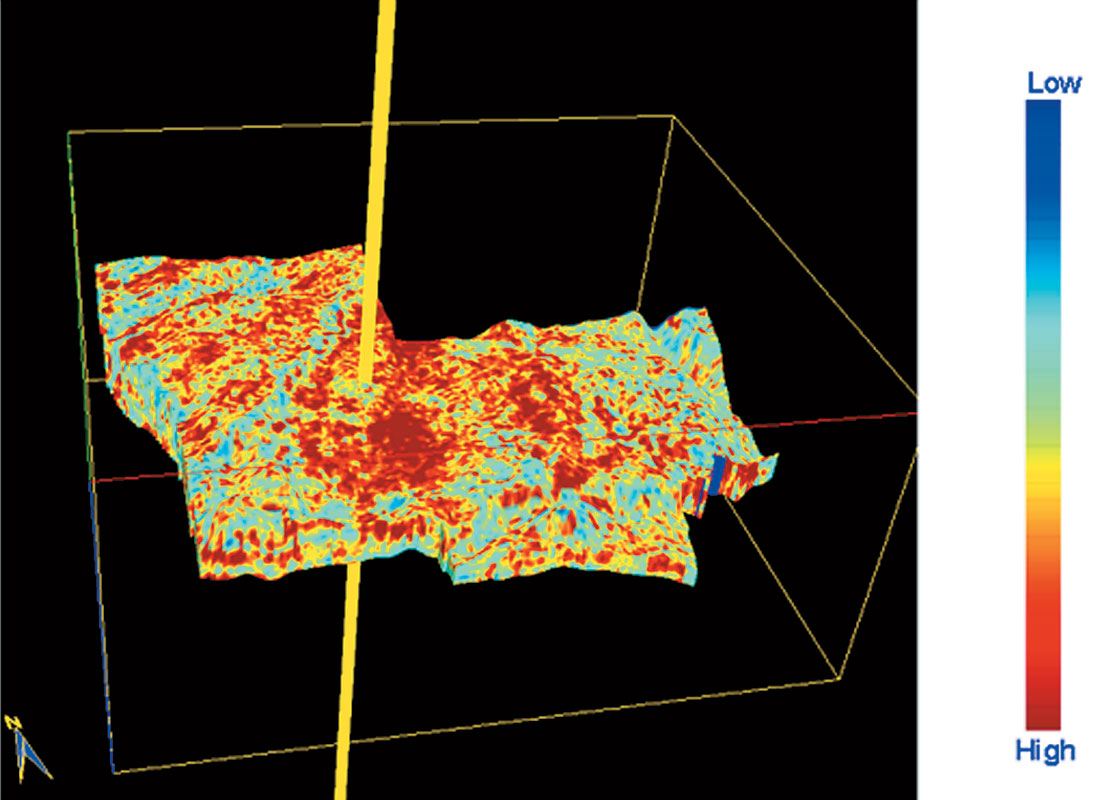
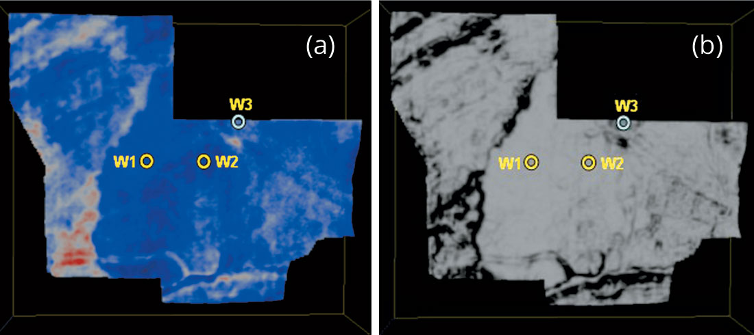
Strat-cube displays are useful for seismic interpreters as they provide them with new insights for studying objects in a 3D perspective, which in turn sheds light on their origin and their spatial relationships. Strat-cubes are subvolumes of seismic data (or their attributes) bounded by two horizons which may not necessarily be parallel. Figure 5 shows a strat-cube display for the energy attribute covering the zone-of-interest and at the level of the reservoir (just below the horizon shown in figure 4). Figure 6(b) shows a strat slice from a coherence volume, processed using a semblance algorithm. While a better definition of some of the subsurface features can be interpreted than in the migrated stack (Fig.6(a)), in this display not much information is forthcoming about the areal extent of the productive sands.

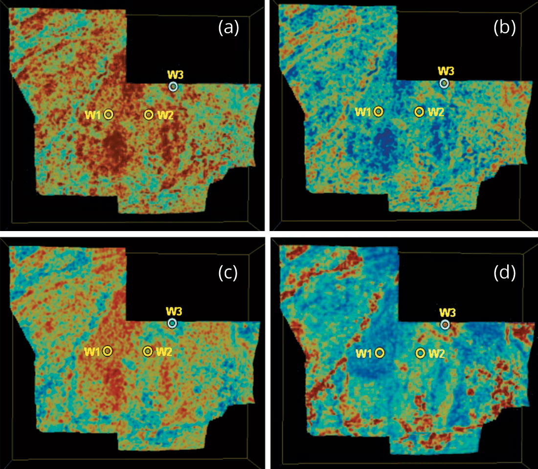
Texture attribute analysis was run on the sub-volume covering the broad zone of interest and figures 7(a) to (d) depict the energy, entropy, homogeneity and contrast attributes. Figure 7(a) shows high values of energy associated with the fluvial deposits and the depicted areal distribution is seen as per expectation. However, this inference needs corroboration with the other texture attributes and we see that in figures 7(b) and (c). High energy in 7(a) is seen associated with low entropy and high homogeneity. Another observation seems interesting here. Well W3 (to the north east of W2) has a different pressure and apparently does not share the same producing formation with W2. The low coherence (figure 6(b)) indicates an island-like feature surrounding this well and the texture attributes confirm this observation. While it is possible to interpret the productive sands on gamma ray logs for wells W1 and W2 (having values less than 50 API units or so), the texture attribute displays provide a more intuitive presentation of the geology – the areal spread of these productive sands.

Case Study 2

The second case study is from south-central Alberta. The objective of acquiring this 3D survey was to explore the possibility of deciding on reservoir pockets that could be drilled. The field has been producing for about a year. Of the 7 wells seen in the area (Figure 8), four are oil wells, two are gas wells, and one is abandoned.

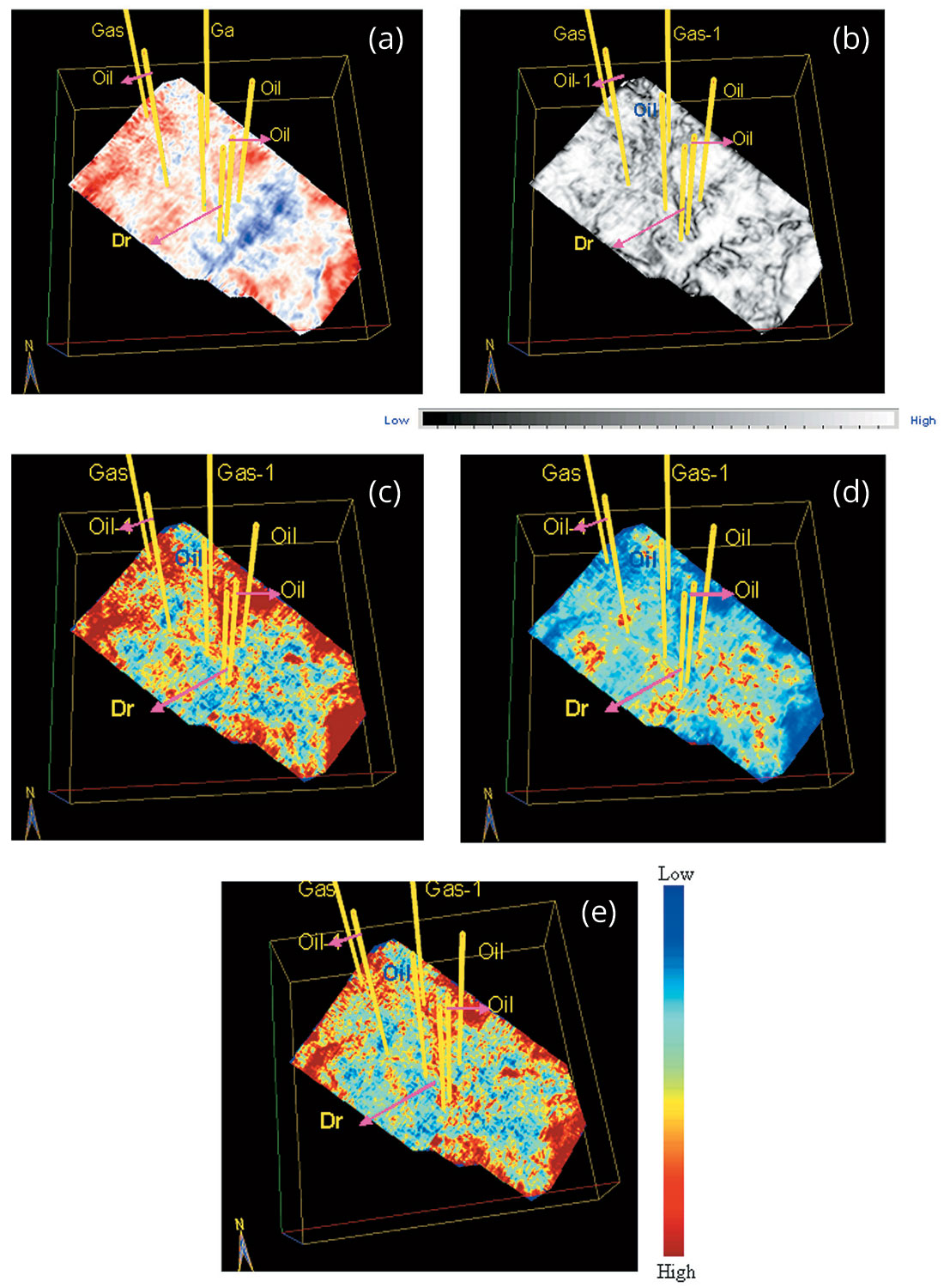
The 3D seismic amplitudes were expected to indicate signatures consistently characterizing the two gas formations, the oil formations could not be detected based solely on amplitudes. However, the seismic data does not help much in this diagnosis. The coherence display indicates several discontinuities at the reservoir level of interest, showing that the reservoir producing formations do not form a blanket but rather are fragmented by way of channels or sand edges seen as these discontinuities. The texture attributes indicate areas that calibrate well for the gas wells. The gas-bearing formations indicate high energy, low entropy and high homogeneity.

The four oil wells are seen associated with moderate values of the energy attribute and the dry well is seen piercing the low energy pocket.

Conclusions

Texture attribute study as presented here is different in that it is not commonly associated with seismic attribute studies. Based on our analysis we find that

1. texture attributes enhance understanding of the reservoir by providing a clearer picture of the distribution, volume and connectivity of the hydrocarbon-bearing facies of the reservoir.
2. texture attributes are a quantitative suite that aids the visual process an interpreter goes through in using the conventional attributes.
3. the simultaneous and exhaustive analysis generating the texture attributes gives insights into how the geology and geophysics and in some cases the engineering properties of the reservoir are linked.

It needs to be mentioned that GLCMs work well for seismic textures as long as the granularity of textures being examined is of the order of the pixel size, and for seismic application this is usually not an issue. Texture analysis depends on the resolution of the data and so the choice of parameters chosen will be important for bringing out patterns of interest.

Acknowledgements

We wish to thank Bashir Durrani for his help in processing of the data shown in Case Study 1, and for helpful discussions. We thank the two companies, who preferred to remain anonymous, for permission to show their data examples. Finally, we would like to thank Arcis Corporation for permission to publish this work.

This paper was presented as a poster at the 2005 CSEG Convention, and it won the ‘Best Poster Award’.