Application of Multiple Regression and Artificial Neural Network Techniques to Predict Shear Wave Velocity from Wireline Log Data for a Carbonate Reservoir, South-West Iran

Abstract

Estimation of shear wave velocity (V_s) using log data is an important approach in the seismic exploration and characterization of a hydrocarbon reservoir. So far all the available empirical models for V_s prediction are mathematical models that incorporate only one or two petrophysical parameters and they lack the generalization capability.

This study has concentrated on the “multiple regression” method and the “neural network” technique to predict V_s from wireline log data. Neural networks can be trained faster to converge the network quickly and without getting stuck in local minima. Neural networks can correlate a stable model for V_s prediction and this is known as “dynamic regression” when comparing with multiple regression.

In this study, after evaluation of the effective petrophysical properties on shear wave velocity, a statistical method was used to establish a correlation among effective petrophysical properties and shear wave velocities. Then a fast training neural net was used to predict V_s from effective parameters. The model is not a ‘black box’-type approach, because we used data from results of multiple regression but it can be easily modified by incorporating adequate V_s data. The established method can predict shear wave velocity from petrophysical parameters and any two of compressional wave velocity, porosity and density, in carbonate rocks with correlation coefficients of about 0.94 for multiple regression and 0.96 for the generalization stage of neural net.

Introduction

The natural complexities of petroleum reservoir systems continue to provide a challenge to geoscientists. The absence of reliable data leads to an inadequate understanding of reservoir behavior and consequently to poor predictions. In past decades, classical data processing tools and physical models were adequate for the solution of relatively simple geological problems. We are increasingly being faced with more complex problems, and reliance on current technologies based on conventional methodologies is becoming less satisfactory (Wong and Nikravesh, 2001).

There are many applications for shear wave velocities in petrophysical, seismic and geomechanical studies. In many developed oil fields, only compressional wave velocities may be available through conventional sonic logs or seismic velocity check shots. For practical purposes such as in seismic modeling, amplitude variation with offset (AVO) analysis, and engineering applications, shear wave velocities or moduli are needed. In these applications, it is important to extract, either empirically or theoretically, the needed shear wave velocities or moduli from available compressional velocities or moduli (Wang, 2000).

In rock physics and its applications, three methods are used normally to study the elastic properties of rocks: theoretical and model studies, laboratory measurements and investigations, and statistical and empirical correlations (Wang, 2000). Multiple regression is an extension of the regression analysis that incorporates additional independent variables in the predictive equation (Balan et al., 1995).

Artificial neural networks are adaptive and parallel information- processing systems that have the ability to develop functional relationships between data and provide a powerful toolbox for nonlinear, multidimensional interpolations. This feature of neural nets makes it possible to capture the existing nonlinear relationships that are most of the time not well understood between input and output parameters (Silpngarmlers et al., 2002). Major applications of neural networks are in seismic inversion, log analysis and 3D reservoir modeling. The applications include determination of lithology, porosity, permeability and fluid saturation from wireline logs and the generation of synthetic wireline logs (missing and unconventional) from other (conventional) logs (Wong and Nikravesh, 2001).

During the past years, many studies have been done on elastic wave velocities focused on related petrophysical properties of rocks. Unfortunately, most of these studies are about sandstones. In Iran most reservoirs are carbonate rocks and thus more study on the petrophysical parameters for carbonates are needed.

In the studied area which is a carbonate oil field in Zagros Basin, south Iran, there isn’t any well with shear wave velocity (V_s) data, thus prediction of V_s from other logs was necessary. Even when an S-wave log has been run, comparison with its prediction from other logs can be a useful quality control.

In this study, a statistical method was utilized to create a correlation among effective petrophysical properties and shear wave velocities in carbonate rocks. The introduced method can estimate V_s with correlation coefficients of about 0.94 for multiple regression and 0.96 for the generalization stage of neural net.

Data Sources

A data set of both compressional and shear velocities in 35 carbonate core samples was used, of which 23 are limestones and remaining are dolomites. The velocities are measured at both dry and water saturated conditions. These data were gathered at an ultrasonic frequency of 0.5-1 MHz.

X-ray diffraction (XRD), thin sections and scanning electronic microscopy (SEM) are used to determine mineralogy, volume of individual minerals and other microscopic sedimentological features. The petrophysical properties of these core samples cover a wide range for exploration interest, with porosity from 0.2% to 29%, permeability from 0.02 to 228.2 mD, clay content from 0% to 10%, calcite content from 47% to 98% and dolomite from 0% to 49%.

Petrophysical wireline log data were gathered from four wells and after deletion of bad hole data, all data are environmentally corrected and of course with comparison of core porosity these logs were depth matched.

Shear Wave Velocity Predictor

In the development of the V_s predictor, 35 samples of V_s were collected. These data were used for multiple regression to establish a model for V_s prediction and because we did not have enough data to train the network, some data sets that were created from multiple regression were used during the training stage, while the other sets were preserved to test the prediction ability of the model.

Input Parameters

Because of the difficulty in finding V_s values along with all rock and fluid properties, only the most commonly reported and easily measurable rock and fluid properties that can be obtained from wireline log, were selected as the main input parameters to the model. These selected parameters must also have significant influence on the V_s.

In order to find effective parameters on V_s, we can study empirical equations that incorporate various petrophysical parameters to predict V_s. There are several empirical equations (for example, Han et al., (1986) and Castagna et al., (1993)) to predict V_s from other logs. Due to high validation of V_p-V_s relationships in carbonate rocks, we apply only the Castagna equation and other parameters and their influence will be distinguished from crossplots for these parameters and V_s.

In general, these empirical relationships give good results only in similar formations and their reliability for other rocks should be considered suspect until a calibration is established. It is therefore useful to have a physical model that provides some understanding of shear wave behavior (Wang, 2000).

Although the prediction should be the same, if all measurements are error free, comparison of predictions with laboratory and logging measurements show that predictions using compressional wave velocities are the most reliable, especially for carbonate rocks. Figure 1 shows a good relation between V_p and V_s in well No. 3 for samples measured under water-saturated condition at 31-33Mpa effective stress. Figure 2 shows the plots of predicted V_s, using the equation proposed by Castagna et al., (1993), versus measured data for water saturated samples. Notice that the V_p data for this equation are derived from sonic logs. The Castagna et al., equations for limestone and dolomite are:

(1)  V_s (km/s) = - 0.05509V_p ² + 1.0168V_p - 1.0305

(2)  V_s (km/s) = 0.583V_p - 0.07776

where, V_p is in km/s and derived from sonic logs.

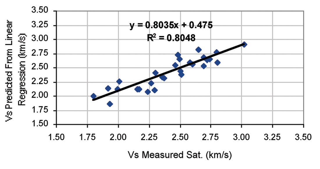
In order to deliver an equation with a better correlation coefficient (Castagna et al., equation has a correlation coefficient of about 0.70), we used a statistical method to approach a statistical correlation that calculates V_s in this field. At first, we used only V_p from sonic logs as input to the Castagna equation for these carbonate samples. The obtained equation is:

(3)  V_s (km/s) = - 0.1236V_p 2 + 1.6126V_p - 2.3057

where, V_p and V_s are in km/s. Figure 3 shows the plots of predicted V_s using the equation 3. This equation has one input parameter and correlation coefficient for this equation is approximately 0.80.

Other parameters including Neutron Porosity (NPHI), Bulk Density (RHOB), Gamma Ray (GR) and deep laterolog (LLD) were considered for inclusion to the presented equation in order to increase the accuracy of predicted V_s using multiple variable regression. Figures 4 through 7 show the effect of porosity, clay content, bulk density and deep resistivity on V_s. Clay content is a significant factor in the study of acoustic velocities. Due to a low amount of clay content of the studied samples (mainly less than 6%), the results suggest that clay content had a negligible effect on velocity. V_s decreases with increasing porosity and deep resistivity and increases with increasing bulk density.

Multiple Regression

Multiple regression is an extension of the regression analysis that incorporates additional independent variables in the predictive equation (Balan et al., 1995). However, the previous empirical studies provide the guidelines for selecting the dependent variables which are to be used in the predictor development. A different predictive equation must be established for each new area or new field.

Now, we can use five parameters that were mentioned before (V_p, neutron porosity, bulk density, deep resistivity and Gamma ray) as input to multiple regression.

A multivariate model of the data solves for unknown coefficients a₀, a₁, a₂,…, a₅ of a multivariate equation such as equation 4:

(4)  V_s = a₀ + a₁ V_p+ a₂ NPHI+ a₃ RHOB+ a₄ GR+ a₅ LLD

The weight of the input variables to predict V_s is given by their degree of contribution to the V_s , which is determined by the multiple regression. Contribution factors (3.28, 0.4380, -1.3820, - 1.0544, 0.0037 and -0.0011 respectively for a₀, V_p, NPHI, RHOB, LLD and GR) indicate that the most important variables in this regression are the NPHI, RHOB and V_p. The weakest variables are the GR and LLD. This means that they may be taken out of the model as in this case, R2 was nearly 91% when all parameters were used. We omitted these two factors, GR and LLD and added the power of other two effective factors and then R2 increased about three percent and reached to 0.94. The new equation is as follows:

(5)  V_s = -17.0885+0.4068*V_p-2.1907*NPHI2-1.1794*NPHI- 3.2747*RHOB²+15.3587*RHOB

Estimated V_s using equation 5 shows a good match with measured V_s (Fig. 8) with R² of about 0.94. Figure 9 presents the computed V_s from multiple regression and V_s from core versus depth for well 3. The results were considered to be slightly better than those obtained from linear analysis. Multiple regression presented a robust correlation to predict V_s from wireline log data. Multiple regression is an extension of the regression analysis that incorporates additional independent variables into the predictive equation .

Both methods, empirical and multiple regression were applied to log data to predict V_s for the studied carbonate reservoir. The result shows that statistical methods perform better than empirical models.

Network Design and Development

Artificial neural networks are parallel distributed information processing models that can recognize highly complex patterns within available data (Mohaghegh and Ameri, 1995). An artificial neural network is an information processing system that has certain performance characteristics in common with biological neural networks and therefore, each network is a collection of neurons that are arranged in specific formations. The basic elements of neural network comprise neurons and their connection strengths (weights). Neurons are grouped into layers. In a multi-layer network there are usually an input layer, one or more hidden layers and an output layer (Mohaghegh, 2001).

The layer that receives the inputs is called the input layer. It typically performs no function on the input signal. The network outputs are generated from the output layer. Any other layers are called hidden layers because they are internal to the network and have no direct contact with the external environment. Sometimes they are likened to a “black box” within the network system. However, just because they are not immediately visible does not mean that one cannot examine the function of those layers.

The ‘topology’ or structure of a network defines how the neurons in different layers are connected. In this case we have three parameters (neutron porosity, bulk density and transit time-DT) with significant influence on V_s. Variables such as Gamma Ray, deep laterolog, X and Y coordinates can provide valuable information to the network, thus were used as input parameters (Figure 10).

A mathematical function then combines the input with some ‘prior’ connection weights (initial weights); it applies an updating algorithm, and produces the final weights after a number of iterations, when a performance criterion is achieved. This process is often referred to as “learning”.

Learning can be performed by “supervised” or “unsupervised” algorithms. The performer requires a set of known input-output data patterns (or training patterns), while the latter requires only the input patterns (Wong and Nikravesh, 2001).

In a typical neural data processing procedure, the data base is divided into two separate portions called training and test sets. The training set is used to develop the desired network. In this process, the desired output in the training set is used to help the network adjust the weights between its neurons (supervised training). Once the network has the learned information in the training set and has ‘converged,’ the test set is applied to the network for verification. It is important to note that, although the user has the desired output of the test set, it has not been seen by the network. This ensures the integrity and robustness of the trained network (Mohaghegh and Ameri, 1995).

In this study, DTs predictors were developed using a back propagation network (BPN), which is one type of feed-forward and supervised neural network using the generalized delta rule, a powerful learning rule. Once the network weights and biases have been initialized, the network is ready for training. The ability of a network to generalize can be developed by training it with different examples and in this study the network can be trained for function approximation (nonlinear regression that has been described in the last section). As was mentioned, during training the weights and biases of the network are iteratively adjusted to minimize the network performance function net (Figure 11). The default performance function for a feed-forward network is average (mean) square error between the network outputs and target outputs that is below a certain tolerance value (in this study, MSE is set to 0.001 it is shown in Figure 12). Once the error becomes smaller than the specified criterion, the network is considered to be trained, the learning process is stopped, and connection weights are fixed. The network is now ready for the testing stage.

Three-layer (input, hidden, and output layers) BPNs were developed as a DTs predictor. A tangent sigmoid function producing outputs in the range of [-1,1] is used as a transfer characteristic for each neuron in the hidden and output layers. The tangent sigmoid is used because inputs are normalized within this range (Figure 13).

BPNs are probably the most well known and widely used networks among the current types of neural network systems available. Even though the back-propagation algorithm is powerful and simple to implement, BPNs have some drawbacks, such as slow convergence and the possibility that the network converges to a local minimum. Some improvement can be made to overcome these drawbacks. The rate of convergence can be affected by a learning rate that determines how fast a network will learn relationships between input and output patterns. The learning rate has a value between 0 to 1. The smaller the value of the learning rate, the slower the learning process will be. Adjusting the learning rate during the course of training can accelerate the convergence. One approach is varying the learning rate during the training stage (Silpngarmles et. al., 2002) and in order to apply a varying learning rate, we can choose a faster training such as variable learning rate (such as ‘traingda’ or ‘traingdx’ in Matlab software).

These faster algorithms fall into two main categories:

1. Heuristic techniques that developed from an analysis of the performance of the standard steepest descent algorithm such as variable learning rate BPNs.
2. Standard numerical optimization techniques such as conjugate gradient and Leverberg Marquardt algorithms.

In standard BPNs the learning rate is held constant throughout training and so is very sensitive to the proper setting of the learning rate. Furthermore, this algorithm is often too slow for practical problems. In faster training, we have algorithms that can converge faster than standard algorithms. In the variable (adaptive) learning rate algorithm, the learning rate is decreased (typically by multiplying by lr-dec equal to 0.7) if the new error is less than the old error (global error increases) and learning rate increased (typically by multiplying by lr-inc equal to 1.05). When the learning rate is too high to guarantee a decrease in error, it gets decreased until stable learning resumes. Figure 11 shows a flow diagram of this algorithm. Another approach to prevent the network getting stuck in a local minimum is to incorporate a momentum term that tends to accelerate coverage when the weight vector is moving in a consistent direction (momentum has a constant value between 0 and 1 and we choose 0.7 for it). This training continues until the average error decreases below 0.001.

When the training is completed, the network is tested for its learning and generalization capabilities. The test for its learning ability is conducted by testing its capability to produce outputs for the set of inputs that was used in the training. For this purpose about 10% of inputs from the training data have been selected and it is observed that outputs with the desired outputs of this data (have a correlation coefficient of about 0.972).

The test for its generalization ability is carried out by investigating its capability to predict the output sets that were not included in the training process. In this study, for test network generalization, we plot output sets and desired outputs of data that have been chosen for this stage of network development. This plot has a correlation coefficient of about 0.96 between output sets and desired outputs (Figure 14). Figure 15 shows V_s from core and V_s from neural network prediction.

Results and Discussion

In this study, 35 carbonate core samples, from four wells, were used. V_p, V_s, porosity and permeability have been measured for all samples. At first, parameters that have significant influence on V_s were determined and all samples were used to develop the multiple regression. Variables used for the ultimate equation were V_p, bulk density and neutron porosity (equation 5). The neural network developed used multiple regression equations. The neural network was developed using a back propagation neural network with 10 hidden neurons in the middle layer, and logistic activation function (tangent sigmoid) in all hidden and output neurons.

The multiple regression method gave good results during the application phase, but where it is applied to new wells (the data from wells that have been put aside) it usually faces problems. Such problems can be avoided with intelligent solution techniques. Neural networks have abilities to adapt data that has been presented to them in the form of input-output patterns. This characteristic of neural networks has earned them the title of “dynamic regression” when compared to rigid regression methods.

Figure 16 shows V_s from core, multiple regression and neural network methods. As can be seen a good agreement exists between these methods. We did not have a black box (the mathematical relationship between input-output data was introduced to the network) in this study, but the excellent results indicate that training the network was done successfully, especially with the use of faster training methods.

It seems that neural networks, with their ability to discover input-output relationships will increasingly be used in engineering applications, especially those in petroleum engineering usually associated with a high inherent complexity.

Conclusion

This petrophysical study has investigated the use of laboratory measurements of acoustic properties on core samples for prediction of shear wave velocities using sonic logs. In this study all three methods, empirical (only one robust model), multiple regression, and neural network, were applied to log data to predict V_s. The results show that the last two techniques perform better than an empirical model, which can be used to obtain an order of magnitude for V_s. The intelligent technique seems to be an ideal tool, if used properly, and enough data is available for training (for V_s prediction). We observed that the most important variable to this regression are the NPHI, RHOB and V_p that play significant roles in the statistical model. The introduced equation can predict V_s with R2 of about 0.94 and 0.96 for an established network in generalization stage. For this network we used one fast training algorithm (variable learning rate) and did not require setting the sensitive parameter such as learning rate. It seems that the faster training rate causes the network to converge as early as possible, and the network will not get stuck in local minima.

From this study we make the following recommendations and believe that future work should:

1. Apply a conventional model to recognize parameters that affect the object parameter.
2. Incorporate both conceptual geological models and expert roles.
3. Develop hybrid intelligent models (neural-statistics) in order to minimize the technique’s individual weaknesses.
4. Optimize the model parameters of the intelligent techniques (e.g. number of neurons in neural networks) using advanced numerical techniques such as evolutionary computing and fast training to easily and quickly converge the network while avoiding local minima.

Acknowledgements

The authors are grateful for support by the NIOC Research Institute of Petroleum Industry (RIPI), Tehran University and Amirkabir University of Technology. The authors acknowledge NIOC Research Institute of Petroleum Industry (RIPI) for their permission to publish this paper.