Anomalous stacking velocities–critique, analysis, explanations and new insights

Summary

A depth velocity model determination is one of the most important problems in seismic processing and interpretation. A velocity model, beyond its initial purpose to obtain a seismic stack, is used for depth conversion and migration, AVO analysis and inversion, pore pressure prediction and so on. Before a well is drilled, seismic data provides the only information for the velocity. From seismic data we can directly determine only stacking velocities, which give us the best image in time domain. Dix’s formula gives us interval velocities in 1-D media. In many cases, the 1D assumption does not work, especially when we have local velocity anomalies in the overburden. Not only do they reduce post-stack image quality, but also create large differences in stacking velocity behaviour for deep seismic reflectors with small dips. In this paper, we will see how we can analytically describe the connection between interval velocities, shallow velocity anomalies and stacking velocities. This connection will provide us with a clearer understanding of the so called “anomalous” behavior of stacking velocities. It also creates a basis for automatic velocity analysis and reflection traveltime inversion in the presence of shallow anomalies.

Introduction to the problem

Many authors have investigated this problem using velocity modeling: Miller (1974), Honeyman (1983), Blackburn (1980), Pickard (1992), Sorin et al (1996), Landa and Keydar (1998). They created some specific depth velocity models, which were important for solving certain geological problems. For each specific geological situation, one can create a particular model, calculate raypaths and time arrivals and see how stacking velocities correspond to real (model) velocities. From this we don’t get much information or general knowledge about the connection between stacking and interval velocities. It’s understandable that the number of specific depth velocity models tends to infinity so it’s very hard to come to specific conclusions using only empirical knowledge. Instead of moving from specific models to general conclusions, we are moving from general theoretical conclusions to particular numerical examples on specific models.

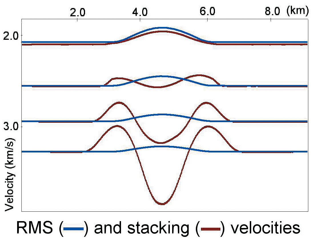
In the presence of a shallow velocity anomaly, we can often see an “anomalous” lateral fluctuation of stacking velocities, increasing with reflector depth. In the 1D case, the stacking velocity is close to RMS velocity, which can be considered as a kind of average velocity. When we think about average velocity, we usually mean that this velocity is bounded by the minimum and maximum interval velocity above. We expect the stacking velocity (many processors in everyday conversation even call it RMS velocity, which is not correct) to behave as a kind of average velocity. That is, if we have a locally slow velocity in some layer, we expect to see slower stacking velocity and vice versa. The thicker a specific layer is, the greater is its influence on the average value. This is true if the velocity anomaly is in a deep layer, but if the anomaly is shallow then the stacking velocity is “spoiled” – it does not correlate with average velocity at all.

As was described above, we often expect stacking velocity to be directly connected with some kind of average velocity over the reflector: “Because one wants the stacking velocities to approximate real velocities”, Blackburn (1980, p. 1466). When we don’t see this connection, we consider this as an error in the stacking velocity. We can see this word “error” in the title of papers (Blackburn, 1980) or in the text of the papers: “In the presence of velocity anomalies, stacking velocities show systematic errors ” Armstrong et al. (2001, p. 81). This “anomalous” behavior even leads to the statements, that “Stacking velocities, as derived from NMO correction of CDP gathers, need have no physical significance to the true velocity distribution below the gather location” Blackburn (1980, p.1466).

The connection between stacking and interval velocities has been considered over the last 50 years by many authors ( reviews of this problem can be found, for example, in Wapenaar and Berkhout, 1985; Bergler et al, 2001) but the formulae (except for media with homogeneous horizontal layers) are quite complicated and require zero-offset ray parameters, which have to be numerically calculated. Moreover, these formulae have been obtained for velocity models with plane boundaries and constant interval velocities, but in the presence of shallow velocity anomalies, the main factors are non-linear changes of the interfaces and interval velocities. That is why all these formulae did not help us to come to some general and very important conclusions.

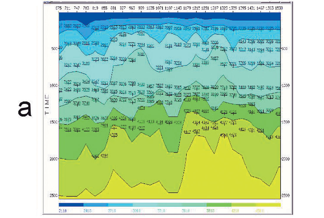
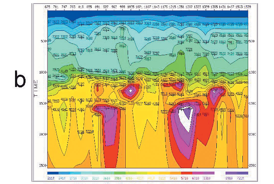
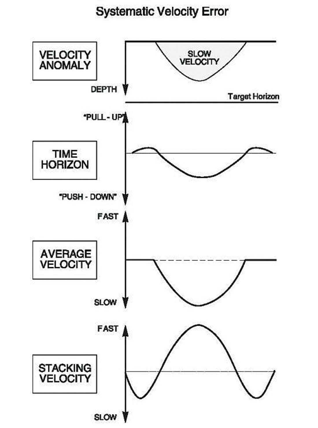
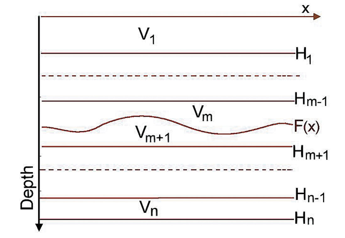
Figure 1 shows the typical behaviour of stacking velocity in the presence of overburden velocity anomalies. Figure 2 is taken from the paper of Armstrong et al, (2001) and the text under this figure says: “A near-surface, slow-velocity anomaly introduces push-down in time at the target horizon on a CMP stack, but the stacking velocity response shows a fast velocity inside the anomaly and slow velocity on either side of the anomaly.” Looking at this picture, we can ask ourselves a question – why do we have this strange behaviour of stacking velocities, which seem to not correspond at all with average velocity?

From the paper by Blackburn (1980) and other papers (Bickel, 1990, Armstrong et al, 2001, Fei and McMechan, 2005, Veeken et al, 2005) we can define several reasons for anomalous stacking velocities:

1. Timing errors as a result of migration
2. Raypath distortion due to the complexity of the overburden
3. Non-flat reflectors
4. Layers with lateral velocity variations
5. Boundary gradient
6. Interval velocity gradient
7. Non-hyperbolic moveout

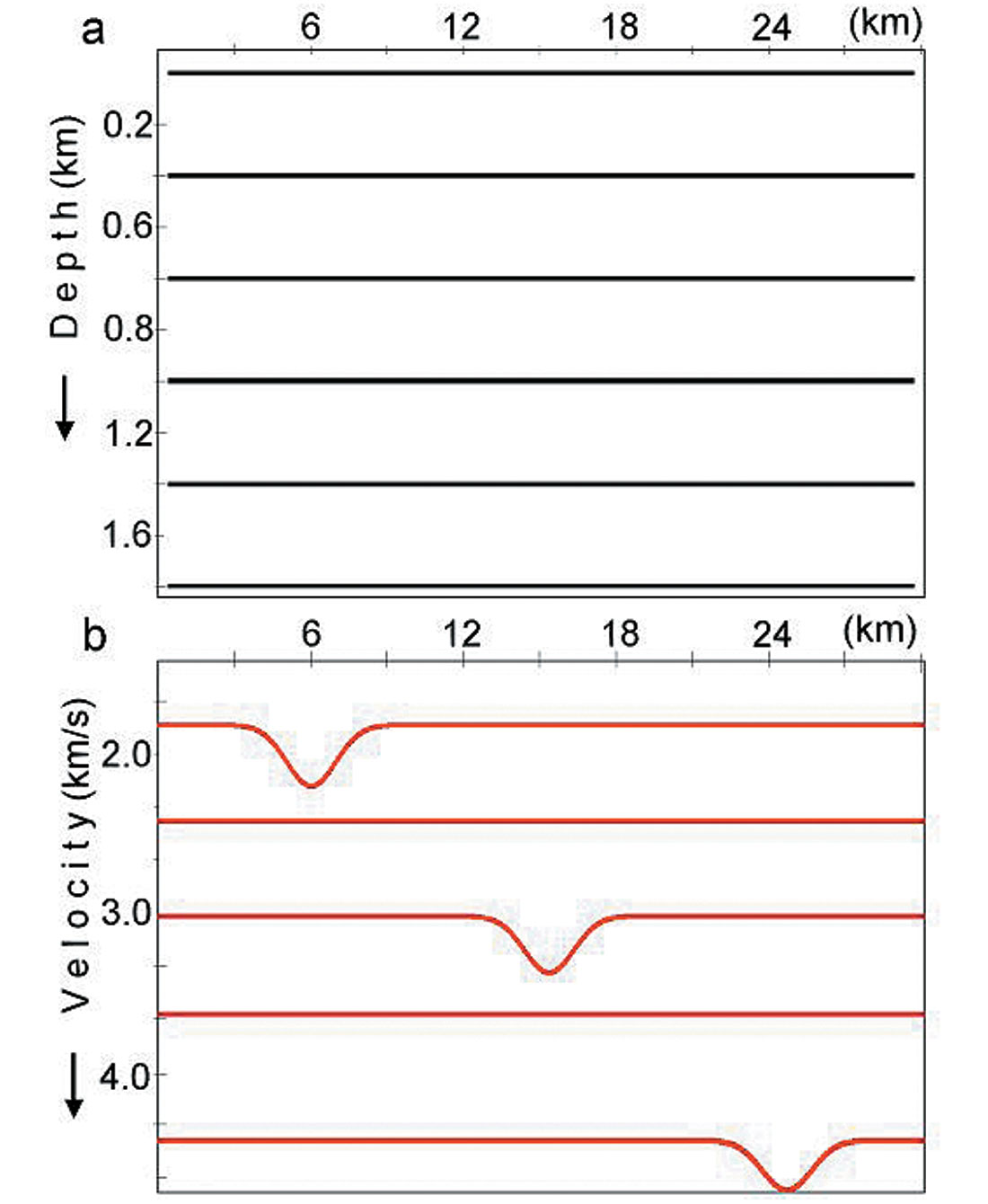
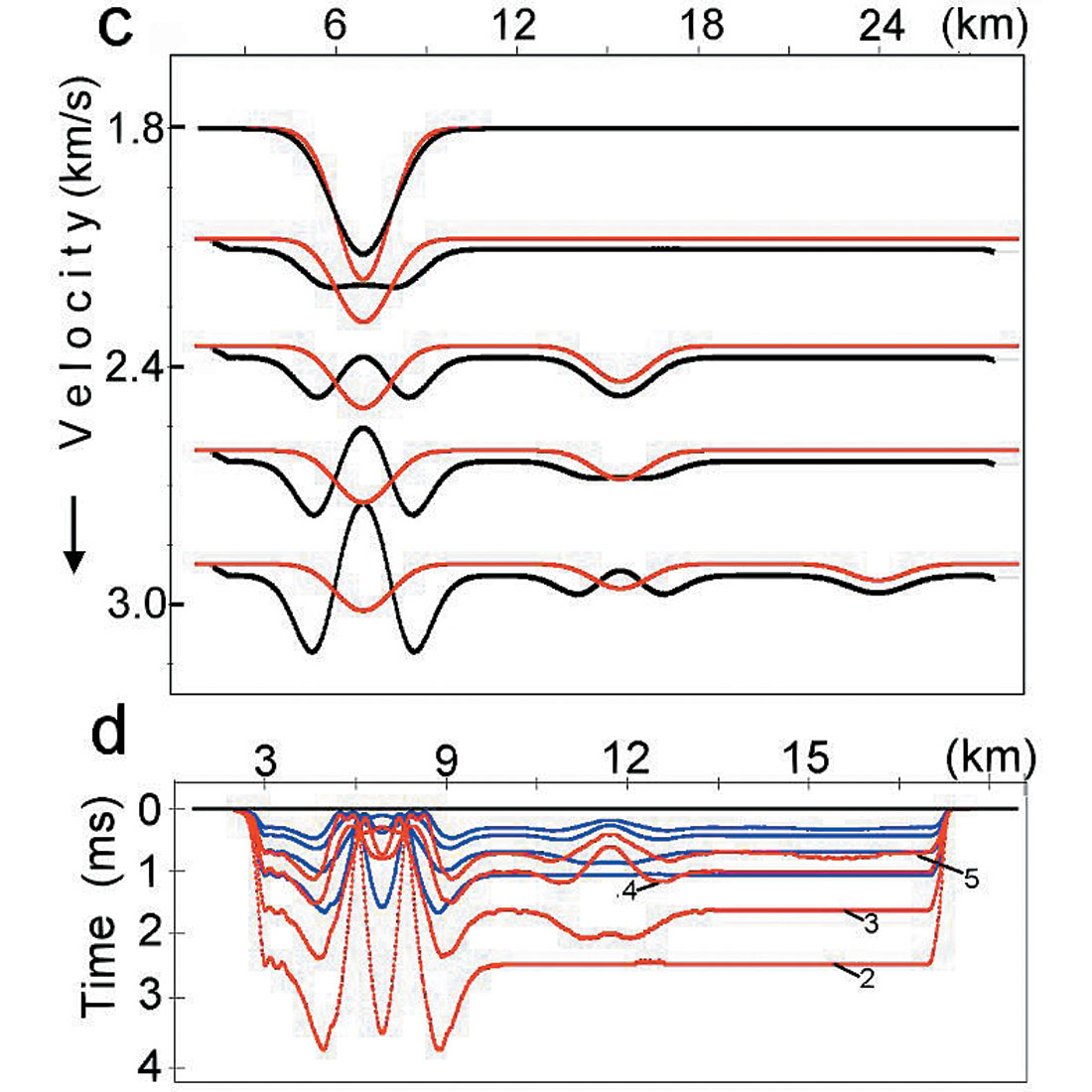
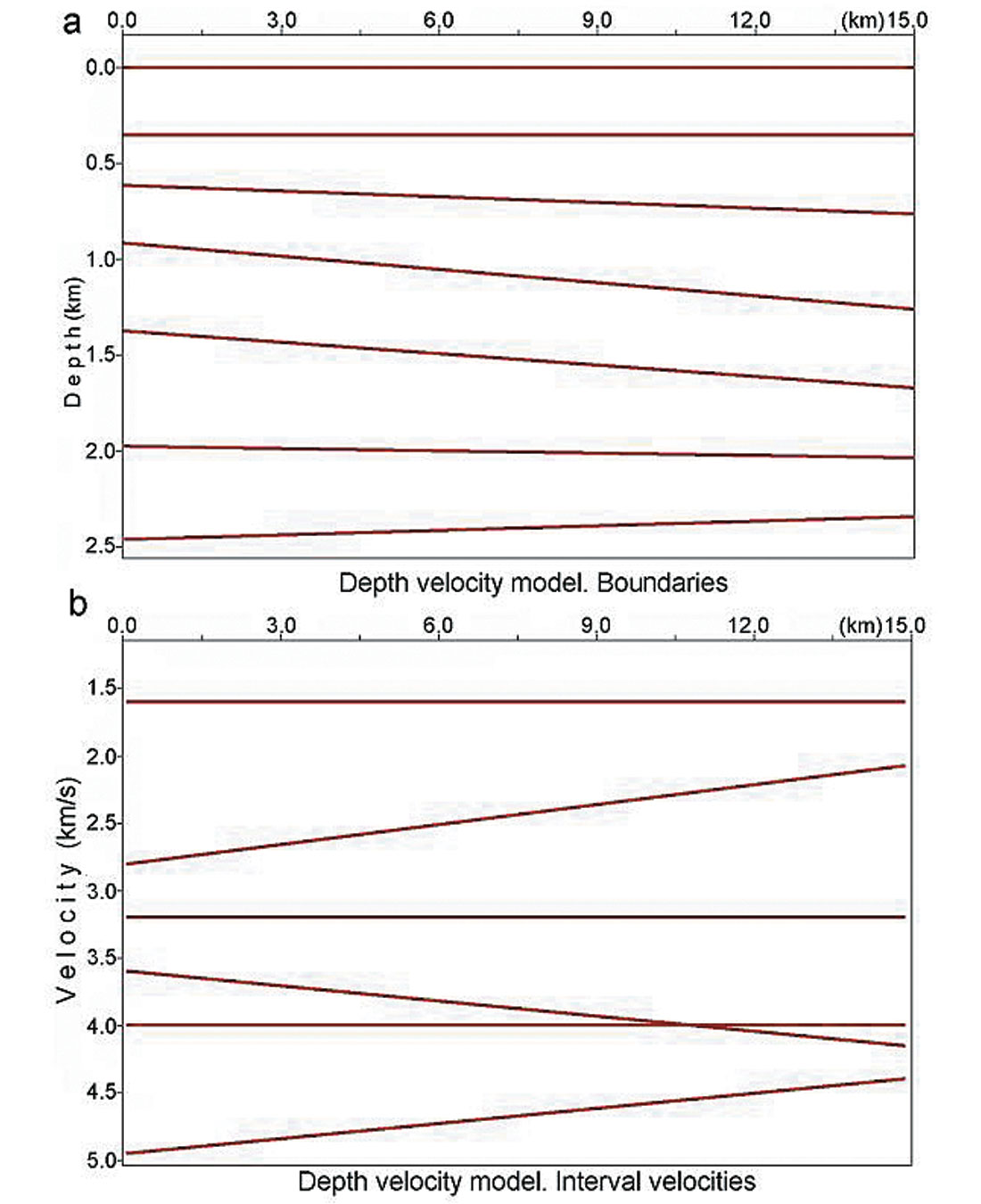
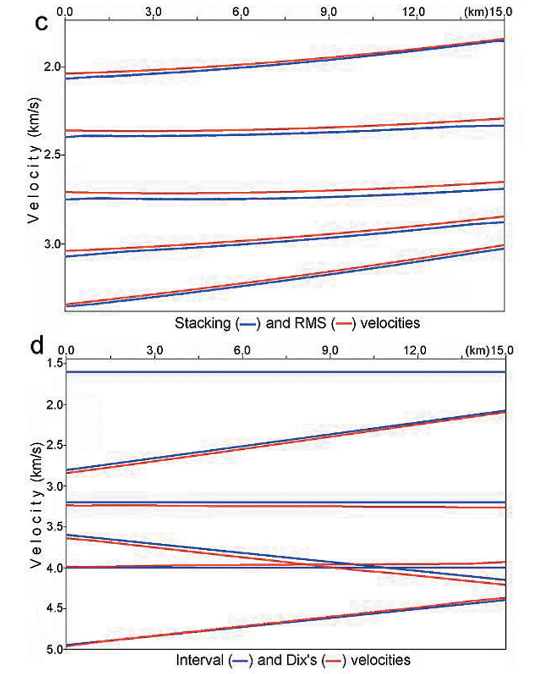
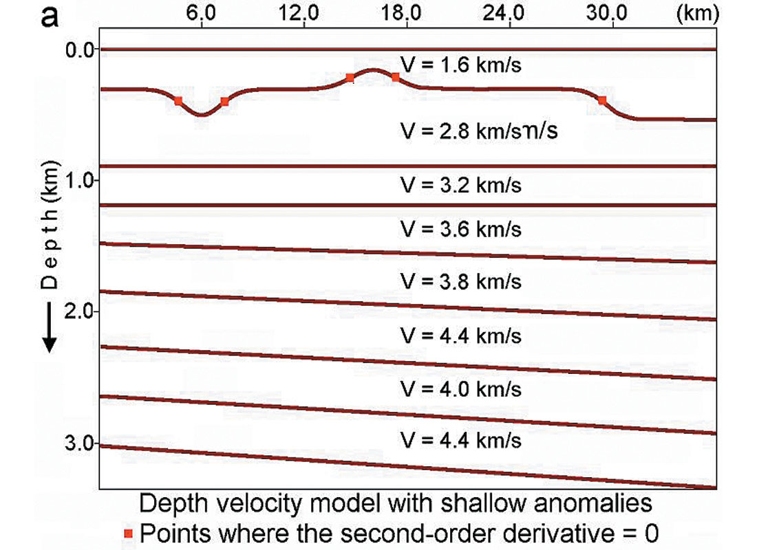
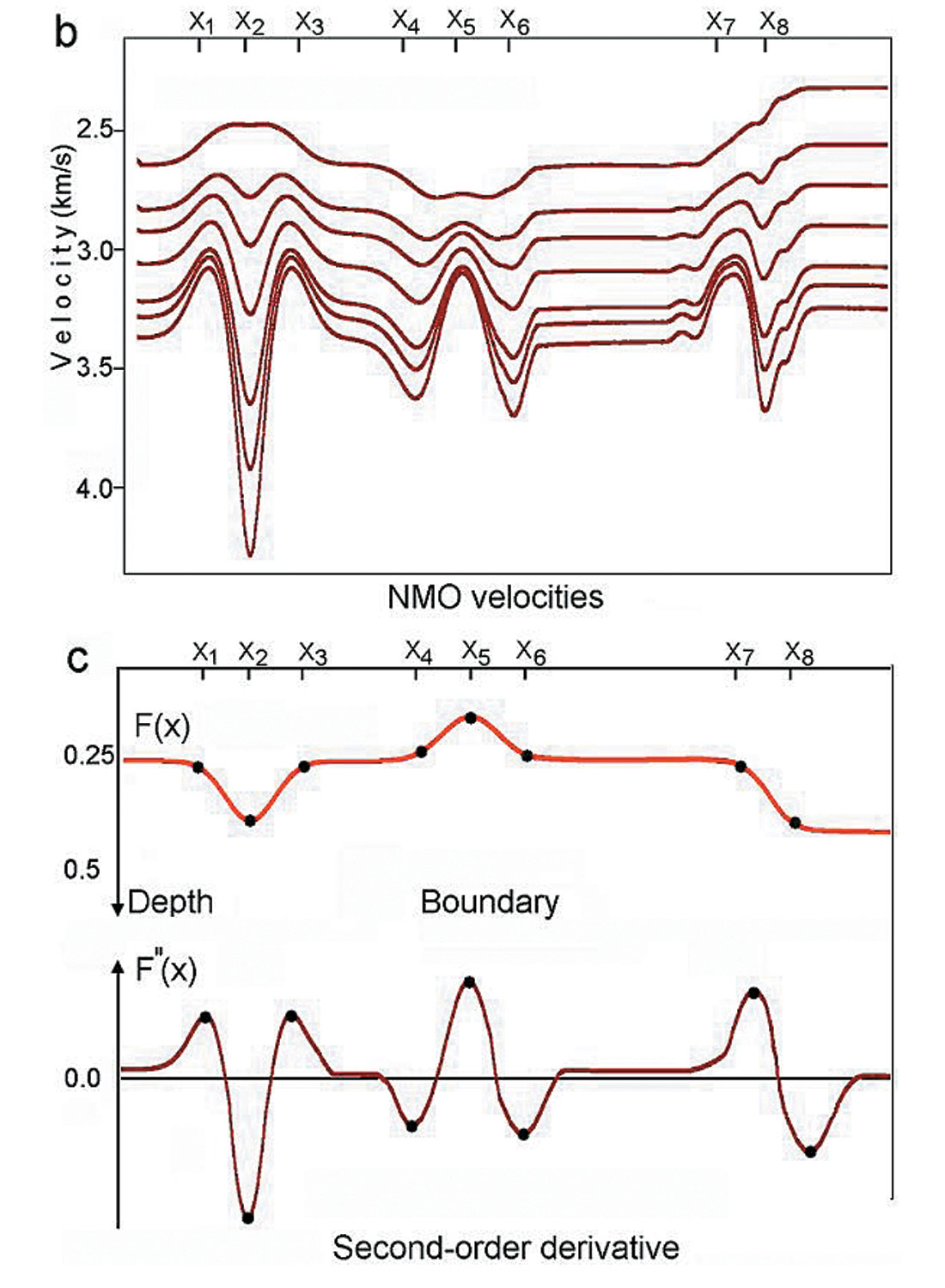
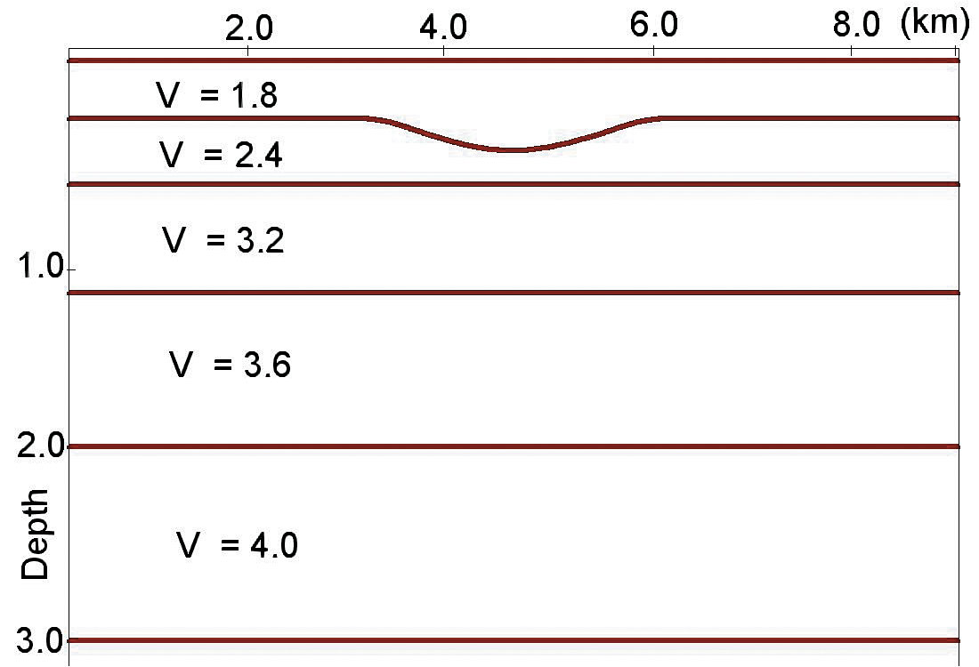
First let’s consider a model example, which shows that even when we have lateral changes in interval velocities, non-parallel beds, non-flat reflectors and migration distortion, Dix formula may give us very accurate results. This means that sometimes we can use a locally 1D velocity model for the subsurface with laterally varying velocities and boundaries. Boundaries for this model are shown in figure 3a, interval velocities are shown in figure 3c by the brown lines. For this model, NMO functions (traveltimes) have been calculated via raytracing.

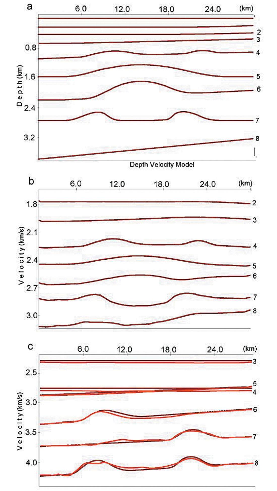
These time arrivals have been approximated by hyperbolas using a spreadlength equal to 0.8 of the reflector depth. The calculated stacking velocities are shown in figure 3b. Dix formula is then applied to these stacking velocities, giving the result as shown in figure 3c by the red lines. We see that even though the subsurface model contains curvilinear boundaries and interval velocities with lateral changes, the Dix formula gives quite accurate results. It implies that for this model stacking velocities are close to RMS velocities and we can use a locally 1-D velocity model when considering interval velocity determination. This modeling shows that items 1 – 6 from above don’t have to cause anomalous stacking velocity behaviour. We will see that non-hyperbolic moveout is not the origin of the anomalous behaviour of stacking velocities either.

We could also ask more questions, such as:

1. Should we consider this “strange” behaviour of stacking velocities as an error?
2. If it’s not an error, what kind of connection can we expect between the stacking velocity and interval velocities?
3. Is this behaviour really caused by non-hyperbolic moveout, as we can find in some papers: “This follows because the origin of the anomalous response is non-hyperbolic moveout within CMP gathers introduced by time delays caused by the velocity anomalies”, Armstrong et al. (2001, p. 82) or is there another reason?
4. Can we use these “errors” to recover shallow velocity anomalies and to build a depth velocity model?

To answer all of the above questions and to explain all of the remarks, we will use explicit formulae, which connect interval and stacking velocity when we have lateral changes in the velocity (Blias, 1981, 1988, 2003, 2005). These formulae are valid for an arbitrary number of anomalous layers, but for the sake of simplicity (and space) we will consider the case of only one layer with a velocity anomaly. To confirm the conclusions, which these approximate formulae imply, we will use several different velocity models. A difference between the use of modeling in this paper and numerical tests in other papers is that we are using models to confirm the conclusions theoretically obtained from the explicit formulae, while in other papers the authors came to some conclusions through the modeling. Because one cannot cover all possible cases with specific models, these empirical conclusions are often not quite complete. Explicit formulae (even if they are approximate and derived with some assumptions) give us a powerful tool to come to some general conclusions, which can be confirmed using model calculations. They give new insights into the reasons for “strange” stacking velocity behaviour, which were empirically mentioned in many papers.

Explicit connection between NMO and interval velocities in the presence of shallow anomaly

First let us know that we can use two descriptions of the lateral velocity anomaly. The first description uses two homogeneous layers, separated by a curvilinear boundary, as in figure 4. We can also use a model with one layer with laterally changing velocity v(x). We will consider both models. For the first model the explicit connection between NMO velocity and interval velocities is given by the formula, derived by Blias (Blias, 1981, 1988). To make it easier to obtain a clearer understanding of this connection, let us simplify the formula for stacking velocities. With some assumptions, we can rewrite this as:

where F is the depth of the curvilinear boundary, H is a reflector depth (Figure 4) and V_AVE is an average velocity for the reflector depth.

This expression gives us an understanding of what can happen with stacking velocities in different situations. We should mention that if we have several local velocity anomalies, we just add the similar terms for each anomaly.

A similar formula can be obtained for the second kind of shallow velocity anomaly description (Blias, 2005)

where s_m(x) = 1/v_m(x) is a slowness in the m-th layer.

These expressions allow us to answer most of the questions (i) – (iv) above. It explains why the influence of the velocity anomaly increases with greater reflector depth (Fig. 1). First scalar in (1) and (2) gives us RMS velocity. If the velocity anomaly is close to the reflector (F is close to H) then the term (1-F/H)² is small and the stacking velocity is close to the RMS velocity. With increasing reflector depth with respect to the anomaly depth, the second term in the square brackets in (1) and (2) also increases, which implies a larger difference between the stacking and RMS velocities.

For deep reflectors, lateral changes of the second scalar in (1) and (2) become more important than the first one, and stacking velocities repeat the second-order derivative of the anomaly. That is, a positive second-order derivative in the centre of anomaly on fig. 2 produces a positive stacking velocity anomaly.

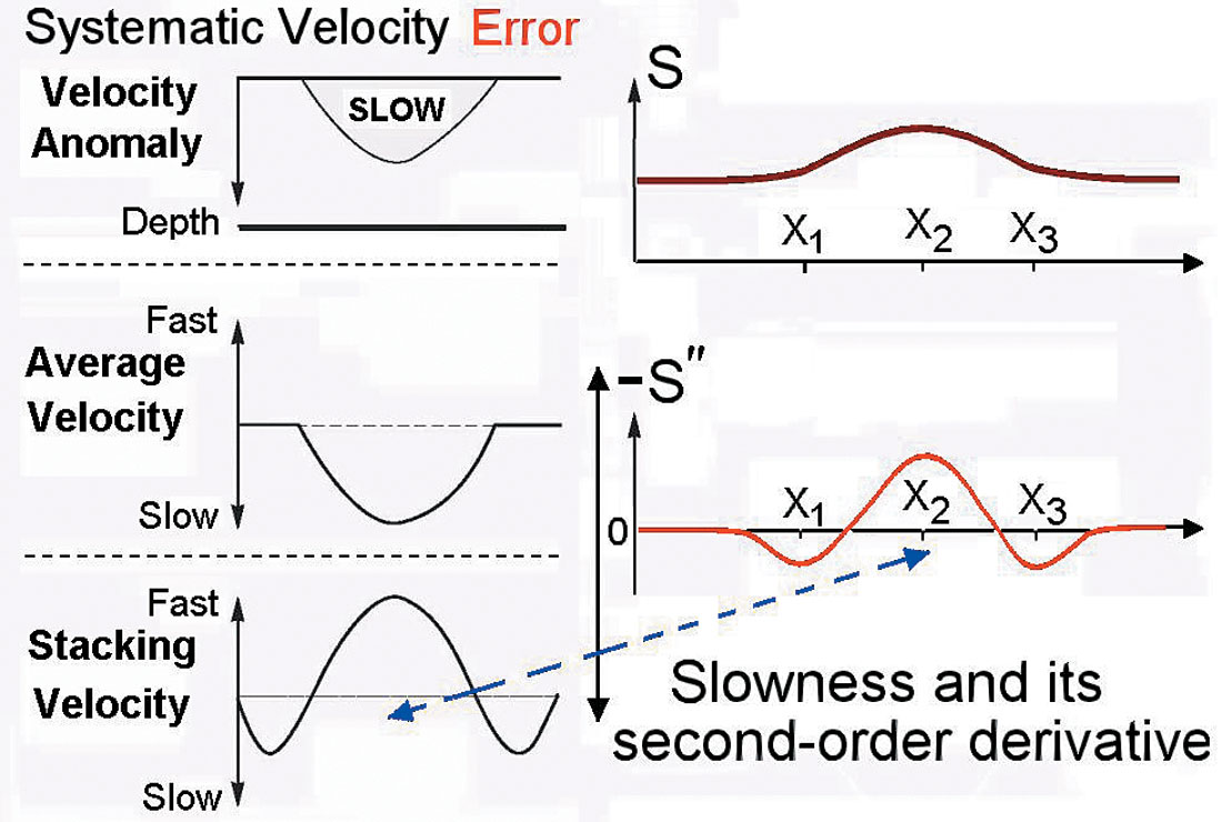
For example, we can now explain the “strange” behaviour of the stacking velocity, shown in the paper of Armstrong et al, 2001. Figure 5 clearly shows the connection between the second-order derivative of the shallow velocity anomaly and stacking velocities. The same theoretical explanation holds for numerical examples considered by Miller (1974), Honeyman (1983) and Pickard (1992).

In conclusion, as stated by Bickel (Bickel, 1990), one can read: “The process of converting stacking velocity to interval velocity is unstable for layers with lateral velocity variations. The instability is due to a long-wavelength ambiguity”. But this is true only for the medium with shallow velocity variations. Lateral velocity changes in the estimated layer do not prevent the use of Dix’s formula. We can theoretically prove this statement using formula (2). If we substitute it into Dix’s formula, after some simple transformation we come to the result:

Here V_Dix is an interval velocity, calculated using Dix’s formula, V_n is an interval velocity in the n-th layer, V_p is velocity in the laterally inhomogeneous layer, H is the reflector depth and F is the depth of the estimated layer. This equation shows that besides thickness of the inhomogeneous layer and non-linear variations of its interval velocity (v“), the difference between Dix’s and interval velocity depends on the difference H-F between the reflector and anomaly depth. This difference is significant if F is small and H is big, that is, if we have a shallow velocity anomaly and deep estimated layer. If we don’t have overburden velocity anomalies then Dix’s formula gives a quite accurate estimation of the interval velocity. This can be confirmed with modeling.

A depth velocity model with horizontal layers is shown in figure 6a, with laterally varying interval velocities given by figure 6b. The resultant RMS and stacking velocities are shown in figure 6c. They show a good fit to formula (2).

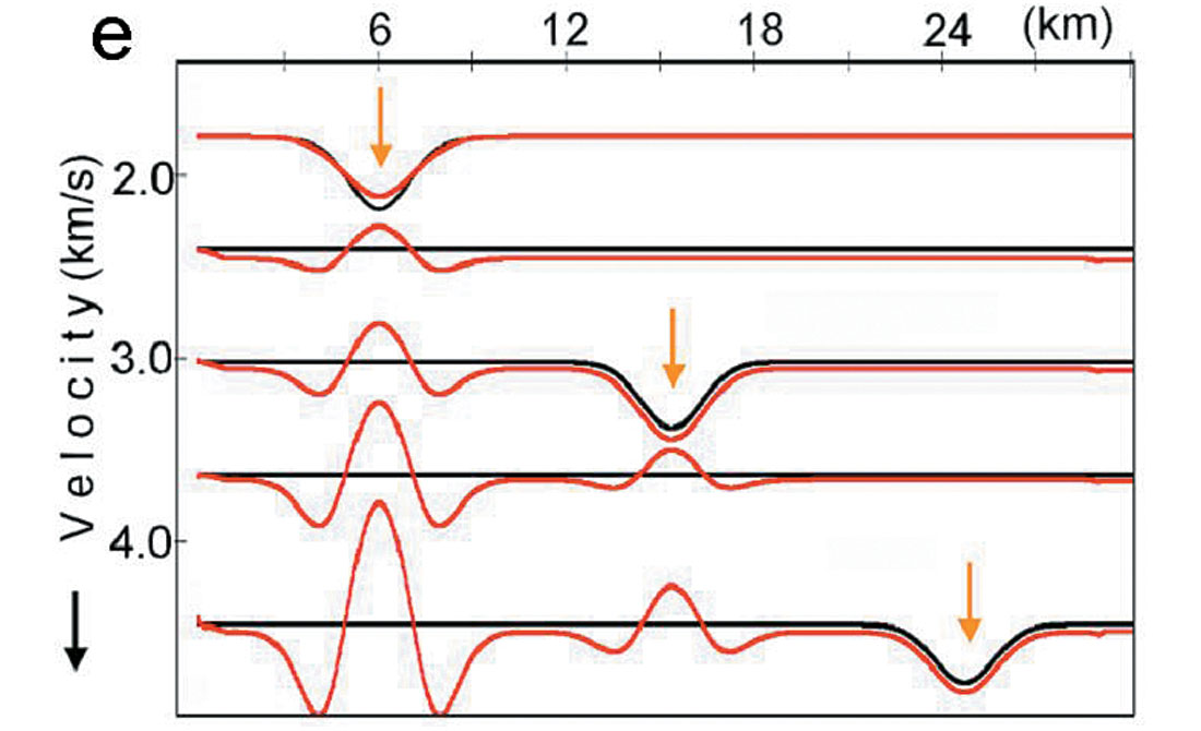
The interval velocities and Dix calculated velocity are given in figure 6e. We see that Dix’s velocity behaviour confirms the theoretical conclusion from formula (3) that if the estimated layer has lateral velocity variations but without an overburden velocity anomaly above it, Dix’s formula works quite well (see yellow arrows). For this model, we have significant (up to 4ms) difference between traveltimes and their hyperbolic approximation (Fig. 6d) but the main reason for interval velocity estimation distortion is non-linear velocity changes over the estimated layer. Though non-hyperbolic moveout can be caused by the lateral velocity changes (or anisotropy), this is not the main reason for an anomalous response. Equations (1) and (2) have been derived for near-zero-offset traveltimes and do not depend on spreadlength at all. It implies that non-hyperbolic moveout is not the reason for anomalous stacking velocity behaviour.

Let’s consider some (but not all) general conclusions from formulae (1) and (2).

(i) First of all, we don’t have the first-order derivatives in (1) and (2); that is linear changes (gradients) in interval velocities and interfaces. This is because we took into account only the first power of the boundary and interval velocity changes. It implies that boundary dips and linear changes in interval velocities (boundary and velocity gradients) do not cause big changes in the stacking velocities. In other words, if we have moderate lateral velocity changes, we should care about non-linear variation rather than the gradient.

Let us demonstrate this property with a numerical example. Figure 7a and b show a depth velocity model with dipping boundaries. RMS (red) and stacking velocities (blue) are shown in figure 7c. We see that stacking velocities are close to RMS, which confirms the above conclusion that moderate linear velocity changes do not imply big changes in stacking velocities and we should pay more attention to the non-linear velocity variations. Figure 7d shows interval velocity (blue lines) and Dix’s velocity (red lines). Here we see that Dix’s formula works well in the area of linear velocity and boundary changes.

(ii) The difference between NMO and RMS velocities depends on the values of the product

for the anomaly, described with the curvilinear boundary, and on the product

if we use lateral variation of the interval velocity to describe a horizontal velocity anomaly. If the value of P is small then the expression in the square brackets in (1) or (2) is close to 1 and the stacking velocity is close to the RMS velocity. Further we don’t have a problem finding interval velocities using Dix’s formula. If the value of P is relatively big then the expression in the square brackets differs from 1 and the difference between the stacking and RMS velocities becomes significant. For deep reflectors, lateral variations of stacking velocities repeat the second-order derivative of the shallow velocity anomaly. These variations are the indicators of the overburden shallow velocity anomalies and can be clearly seen in the stacking velocity grid (Fig. 1).

The NMO velocity can be larger or less than the RMS velocity. It depends on the sign of F“(1/V₁ – 1/V₂):

V_NMO > V_RMS if F“(1/V₁ – 1/V₂)<0;

V_NMO < V_RMS if F“(1/V₁ – 1/V₂) > 0.

It follows that if V₁ < V₂ (we have a low velocity anomaly) then at the points X₁ and X₃ V_RMS < V_NMO because at these points F“ > 0. At the center of anomaly X₂, F“ < 0 and therefore V_RMS is bigger than V_NMO. If we have a high velocity anomaly (V₁ > V₂), the correlation between the stacking and RMS velocities is the opposite.

(iii) Formula (1) shows that there are two factors which influence stacking velocity values. First is the RMS velocity (which we prefer) and the second is non-linear lateral changes in the interval velocity – the anomaly itself. If the reflector depth H is not far from the anomaly depth F then ( 1- F/ H)² is small and the anomaly influence is small. With the reflector depth increasing , the value of ( 1- F/ H)² is also increasing and at some depth it becomes significant. The deeper we go, the less the lateral changes of RMS velocity (as any average velocity) and the larger lateral changes of the value in the square brackets. For deep reflectors lateral changes in RMS velocities are small compared to those of the second order derivatives with large scalars. It leads us to the conclusion that for deep reflectors, the lateral changes of stacking velocity behaviour will be close to the second-order derivative of the SVA (shallow velocity anomaly). To demonstrate this, let’s consider a velocity model with SVA, figure 8a. If we compare stacking velocities for deep boundaries (Fig. 8b) and the second-order derivative for the shallow velocity anomaly boundary (Fig. 8c) we will see that they have the same shape with lateral variations.

While going from shallow reflectors to deep ones, the maximum of stacking velocity in the center of anomaly is changing for the minimum and vise versa. That is what we see in figure 8b. These changes are not the “errors” and they are caused by the second scalar in (1) and (2), which includes the second-order derivatives, that is lateral non-linear velocity changes.

(iv) If there is an elongated velocity anomaly (Fig. 9) then the stacking velocities parallel to the elongation and perpendicular to it will differ significantly. It follows from formulae (1), (2) and the fact that the second-order derivatives will be different in different directions. Along the anomaly, the second-order derivative will be close to zero and stacking velocities will be close to RMS. In the perpendicular direction (transverse to the anomaly) the second-order derivative has significant value and the difference between stacking velocities and RMS velocities can be very large. It implies that in the presence of a shallow elongate velocity anomaly stacking velocities vary in different directions.

(v) Let’s consider an exotic but interesting case. From equation (1) and (2) it follows that the expression in the square brackets can be negative. This means that we will observe reverse time arrivals – minimum time will be at non-zero offset. In this case 1/V_NMO² < 0 so we cannot use stacking velocity at all to describe NMO function. We have to use coefficient b = 1/V_NMO², which is negative for this case. This sounds strange but this is what formula (1) implies and modeling confirms this. Moreover, the proper statement is even stronger: If F“(1/V₁ – 1/V₂) < 0 then there exists such a critical depth, that all horizontal reflectors, deeper than this depth, will create a reverse NMO function. From (1), we can derive an approximate formula for this critical depth:

For most cases this critical depth is too large to see the effects but it is nonetheless possible. Let us consider one model example, which shows the reverse traveltimes for deep reflectors. The depth velocity model is plotted in figure 10a. Figure 10b shows stacking velocities. In the center of the anomaly (around the point X_CDP = 5 km), the NMO functions are reversed. It means that the zero-offset time T(x=0) is a maximum point but not the minimum as it should be in the “normal” case.

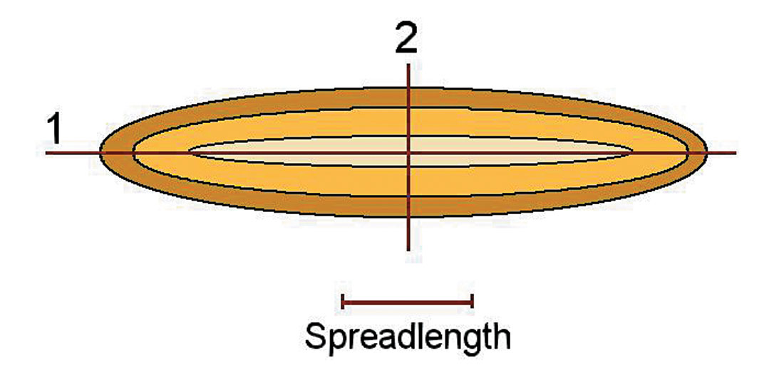
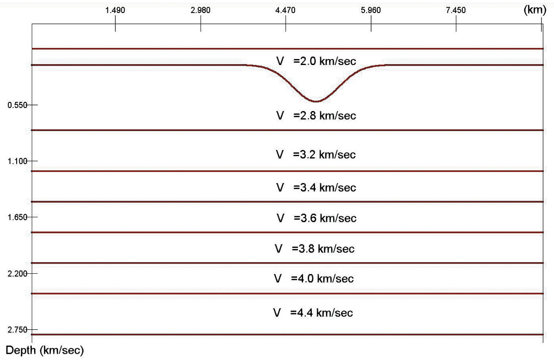
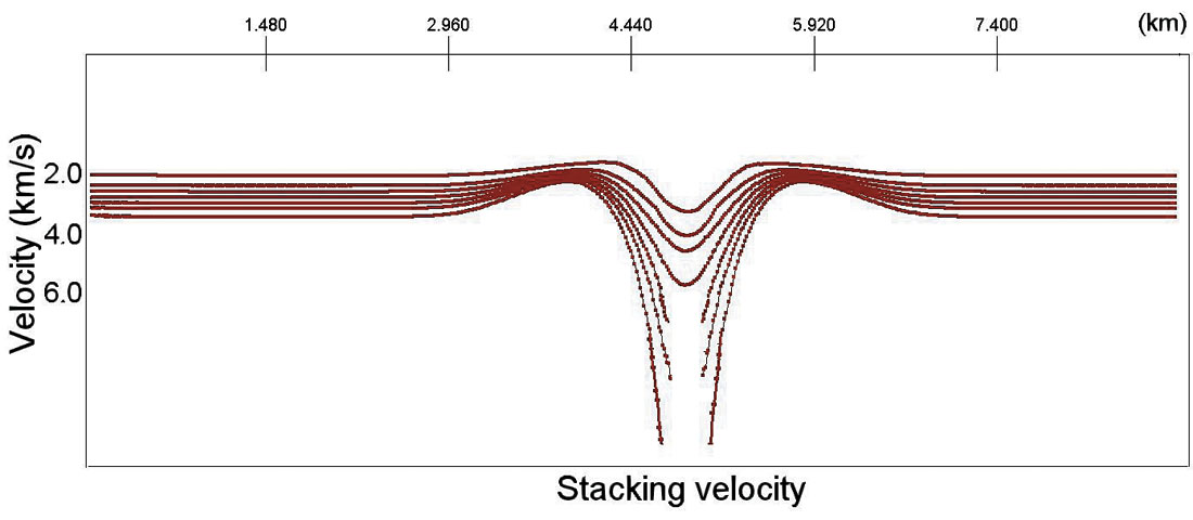
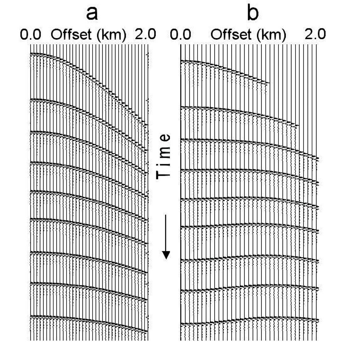
Figure 11 shows CDP gathers in the perpendicular direction. Gathers in figure 11a were calculated at the horizontal line 1 from figure 9. The CDP gathers in figure 11b correspond to the vertical line 2 from figure 9. On the gathers for the vertical line (line 2 across the shallow velocity anomaly), we see that, from deep horizons, the zero-offset trace time is larger than the time for the traces with non-zero offset, as was predicted theoretically. This leads us to the important conclusion that in the case of long elongated overburden velocity anomalies we should run azimuth-dependent velocity analysis for 3D data.

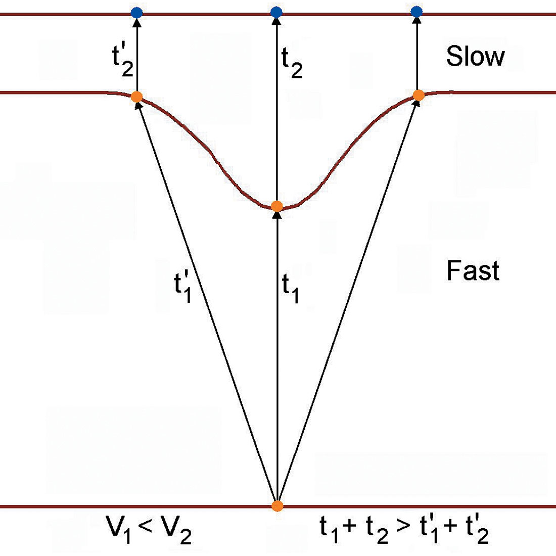
There is a simple physical explanation for this phenomena (Fig. 12). If the velocity in the first layer is low then time t₂ is much bigger than the time t₂’. If below the curvilinear boundary velocity is high then the difference between the times t₁’ and is t₁ less than the difference t₂-t₂’. Then t₁+t₂ > t₁’+t₂’ and this implies that zero offset time is bigger than the offset traveltime.

Here we should touch a migration velocity analysis and prestack depth migration problem. There is no need for prestack migration prior to stacking velocity determination in the presence of a shallow velocity anomaly and relatively small dips of deep reflectors. Prestack depth migration does not help us with the velocity analysis if we have a shallow velocity problem and layers with relatively small dips, less than 10-15°. This was shown on a model example by Sorin et al. (1996). This procedure (building the velocity model through the iterative prestack depth migration) is much more expensive and time consuming than layered traveltime inversion and helps only in the presence of complex deep structures or strong diffracted waves.

(vi) Let us consider extreme points for the NMO velocities at different reflection depths. We rewrite formula (1) and (2), taking into account only first powers of the second terms in the brackets:

where

In formula (4) and (5), the first scalar is RMS velocity, that is the velocity which we have for the locally 1-D medium and for which we can apply Dix’s formula. The second scalar takes into account lateral velocity changes and leads to the anomalous lateral behaviour of stacking velocities. If the reflector depth H is close to the anomaly depth F then Q(H) is small and NMO velocity is similar to RMS velocity. If, for example, we have a low velocity anomaly then NMO velocity will have low values at the same points as the anomaly. At the center of the anomaly, NMO velocity has a local minimum, the same as RMS velocity. If the reflection depth H increases then the value Q(H) also increases and the second term in the brackets becomes large. For deep reflectors, the second scalar in (4) and (5) changes laterally more rapidly then the first one (Fig. 8c) and at the center of the slow velocity anomaly it has a local maximum because F“ < 0 and s_m“ < 0. It implies that, for the deep reflectors, NMO velocity V_NMO also will have a local maximum even though RMS velocity has a local minimum. We come to the conclusion that in the presence of a slow shallow velocity anomaly, stacking velocities have lateral local minimum for shallow reflectors and this minimum changes to maximum for deep reflectors.

To illustrate this let’s consider a velocity model with a slow velocity anomaly in the shallow part of the section,as illustrated by figure 13a. Figure 13b shows stacking and RMS velocities for the reflectors from 2 to 5. We see that for the second boundary (below the anomaly) the stacking velocity is close to the RMS velocity because of a small value of Q(H) in formulas (4) and (5).

Acknowledgements

I would like to thank Michael Burianyk (Shell Canada) for helping with this paper; Dr. Al-Chalabi for his attention and useful discussions. I would also like to acknowledge Valentina Khatchatrian who developed most of the velocity anomaly removal software and Samvel Khatchatrian for useful discussion.