Anisotropic PP and PSv prestack depth migration of 4C seismic data, offshore Trinidad

Abstract

In November 2004, EOG Resources acquired an ocean-bottom cable (OBC) 4C swath survey across the Pamberi-1 well location in the Lower Reverse L block of the Columbus basin, eastern offshore Trinidad. The purpose of the 4C test survey was to evaluate the potential of long-offset multicomponent technology for resolving lithology and stratigraphic detail in an area perturbed by shallow gas, overpressure and illumination shadows from normal regional faults and major anticlinal ridge trends acting as pressure seals. The motivation from EOG for attempting this was because a conventional 3D towed-streamer survey acquired the previous year failed to adequately image the target reflectors comprising the reservoir under the main growth fault.

Details of the P- and PS_v-wave processing of this dataset through anisotropic prestack time migration were previously described (Johns et al., 2006) in which it was demonstrated that there existed a qualitative correlation between derived parameters and attributes from P and S_v anisotropic migration velocities and known regional geology. This observation was quite remarkable considering only a limited effort to constrain or validate parameters (in this case, velocities to the Pamberi-1 well checkshots) was performed. Under the “Future work” section of the previous publication, it was suggested that further data quality enhancement in preparation for more quantitative rock property classification, calibrated to wells, could only be achieved after prestack depth imaging.

In this paper, we present precisely that next phase in the 4C processing, advancing the P- and PS_v-wave data through anisotropic prestack depth migration, using cell-based tomography with a top-down approach. The Pamberi-1 well information was used to constrain the anisotropy in the shallow section, with the deeper, spatial trend away from the proximity of the well determined from the anisotropy derived previously in the time processing.

Prior to proceeding with the anisotropic depth imaging, the magnitude of shear splitting (or, birefringence) from the presence of azimuthal anisotropy (HTI) was first examined to assess its potential impact on the radial rotated P-S signal. The shear-wave splitting analysis revealed a principal angle of polarization that was closely aligned with the regional stress direction delineated by the normal major faults blocks acting as pressure seals.

Introduction

The four-component swath, acquired by WesternGeco’s QSeabed OBC crew at the end of 2004, comprised of two parallel 15-km receiver lines separated by 400m, with a receiver station interval of 25 m. Twelve source lines, with crossline separation of 100 m, were shot into the two cables with a recorded maximum split-straddle offset of 10,000 m and a nominal inline fold of 133.

The 4C survey, situated in the Lower Reverse L block of the Columbus basin, Trinidad, traverses the Pamberi-1 well location. EOG is currently not producing from this well, but consider the location, which is comprised mainly of Plio-Pleistocene sands and shales, to have high prospectivity potential. The objective of the 4C acquisition and processing was to characterize the lithology and reservoir potential of the events directly under the well in the 3,000 to 4,500-m depth range. On previous conventional seismic data this target zone, in the upthrown side of the fault, suffered from a problematic illumination shadow despite the existence of several well-imaged strong reflectors in a downthrown fault trap that form the basis of the prospect.

The original processing, as previously described in detail (Johns et al., 2006) adopted a fairly conventional P- and PS_v-wave signal processing flow prior to imaging through curved-ray Kirchhoff prestack time migration. Data quality was very good with improved imaging at the target level from both wave modes. To match equivalent events the PS section was compressed to P-P time using the derived vertical Vp/Vs ratio (γ0). The preference however, is to process in the depth domain to facilitate the registration of P- and PS_v-wave events in depth through important incorporation of anisotropy calibrated to available well data. Previous papers have been published describing the registration of P- and PS_v-wave data in depth from anisotropic prestack depth imaging. Nolte et al (1999), Crompton et al. (2005) and Kommedal et al. (2006) are a few that exemplify the evolution of the technology. This paper continues in that premise by describing the prestack depth migration (PrSDM) work flow and velocity modeling for P- and PSv-wave data, with inclusion of well control and anisotropy. Results of the final depth migrations are shown compared to the previous prestack time migration (PrSTM).

Before embarking on the anisotropic PrSDM for both wave modes, it was decided to examine and identify the nature of another form of anisotropy, HTI (or azimuthal anisotropy), and its possible effect on PS_v imaging and data quality as a consequence of shear splitting. A proprietary rotation analysis was utilized to extract the principal fast and slow polarization direction from the full elastic shear wave field propagation.

Azimuthal Anisotropy

Azimuthal anisotropy, as opposed to polar anisotropy (VTI/TTI) accounted for in traveltime ray tracing of prestack depth migration, can cause shear waves to split into fast (S₁) and slow (S₂) components, propagating orthogonal to each other. Depending on the difference between S₁ and S₂ and thus the magnitude of azimuthal anisotropy, the polarization could result in reduced resolution of the radial (source-receiver azimuth) PS rotated signal due to the destructive interference of fast and slow shear energy. Numerous papers on shear splitting have been previously published, such as Probert and Kristiansen (2003), which demonstrate the importance of identifying and measuring azimuthal anisotropy on PS data.

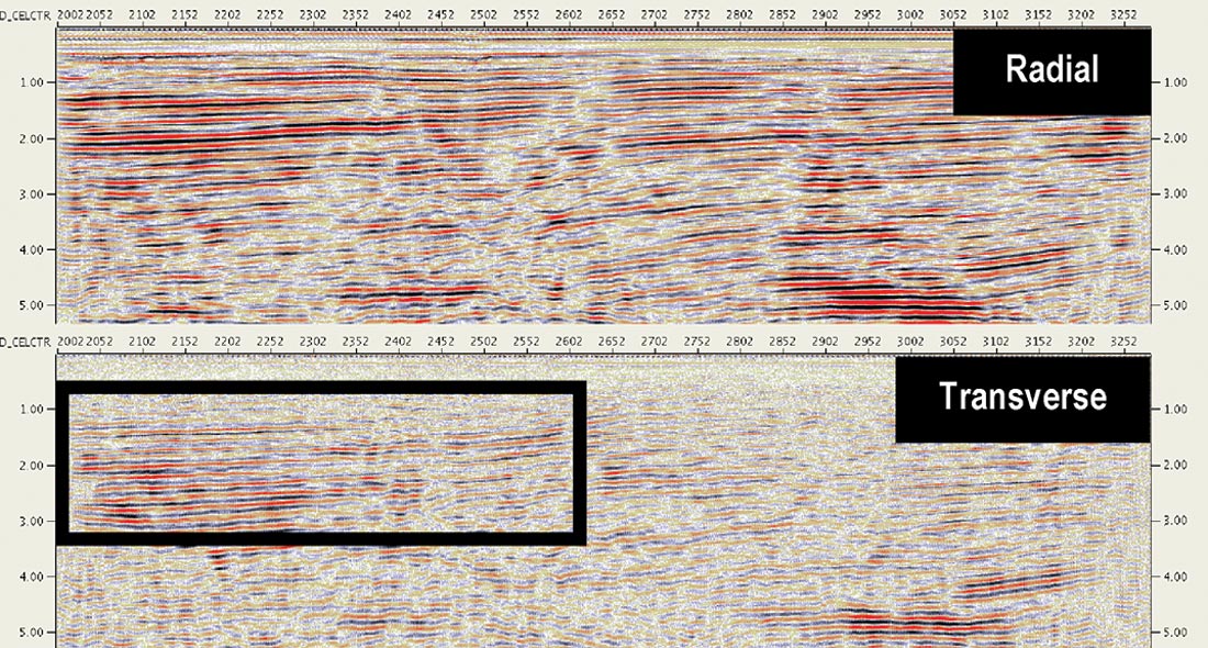
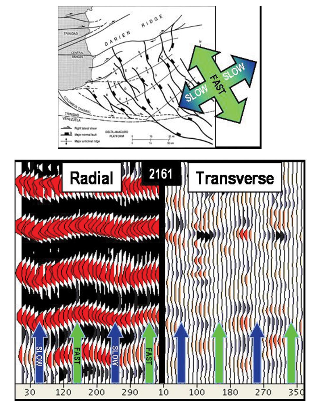
Evidence of shear splitting was initially noted from inspection of the PS radial and transverse QC stacks with simple asymptotic binning. Coherent energy on the transverse section (shown bottom of Figure 1) corresponds to primary reflections seen on the radial stack, implying possible birefringence. The most significant energy is to the left (or southwest end) of the line shown. Detrimental dimming on the radial PS stack is not evident; however it was still considered important to quantify the magnitude of potential shear splitting from azimuth rotation analyses on common receiver gathers. These analyses were performed on 500-m limited-offset 3D azimuth bins, every 1 km, along the northernmost receiver line of the swath. Despite this 4C survey being acquired predominantly inline, the inner 500-m offset range is comprised of a full 3D distribution of azimuths and could be utilized to identify and measure the polarization of the S-wave from analysis of shear splitting.

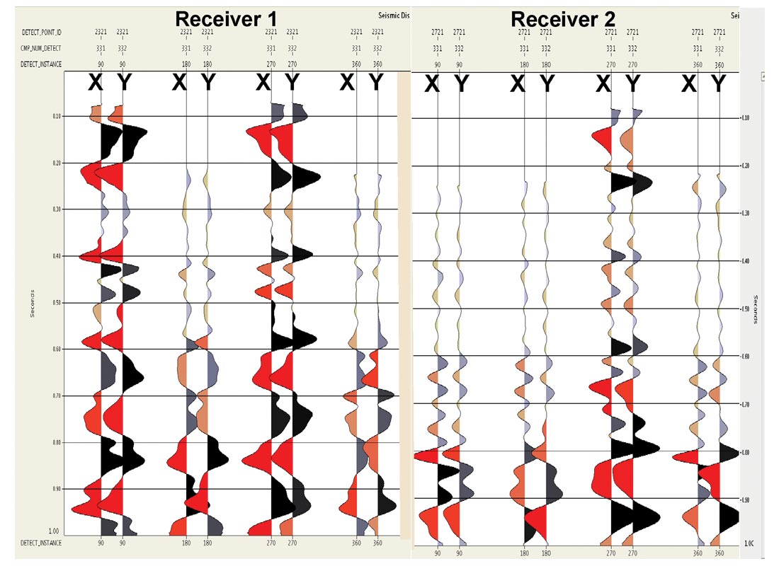
Prior to examining the azimuthal variation on the converted wave data, it was first necessary to verify the vector orientation and fidelity of the OBC detectors, as recorded by the individual geophone accelerometer components, Z, X, and Y. The detector orientation is confirmed by analyzing the relative energy or polarization of the direct arrivals and computing the rotation angle about each of the Z, X, and Y axes. Thereafter, common 45° azimuth traces from each of the horizontal X and Y component receiver gathers are generated (Figure 2) and are found to exhibit impressive correlation, consistent with the OBC system’s reputation for excellent vector fidelity. The visual comparison was so convincing that further hodogram analysis was deemed unnecessary. Part of this analysis process included the derivation of a 3C cross-component equalization operator for matching the Y component to X; an important step utilized commonly for legacy OBC systems. The operator derived on this dataset proved to be consistently close to zero phase for all receivers, and as a result, its application had little effect and was considered unnecessary.

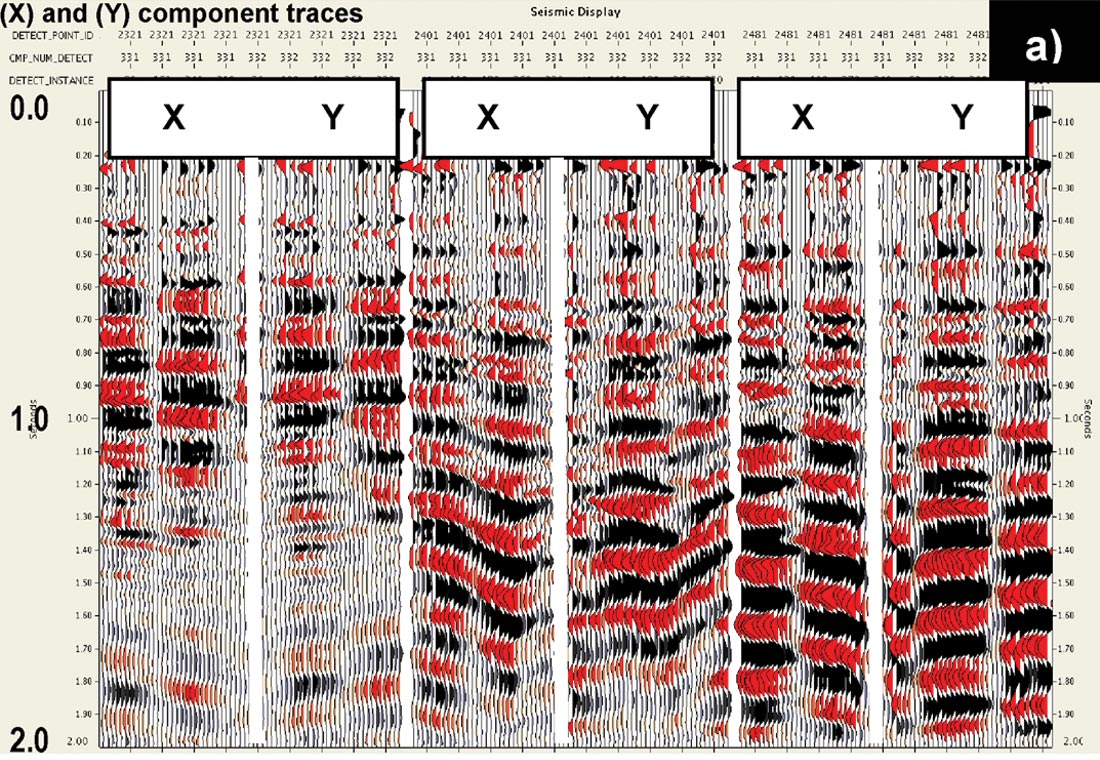
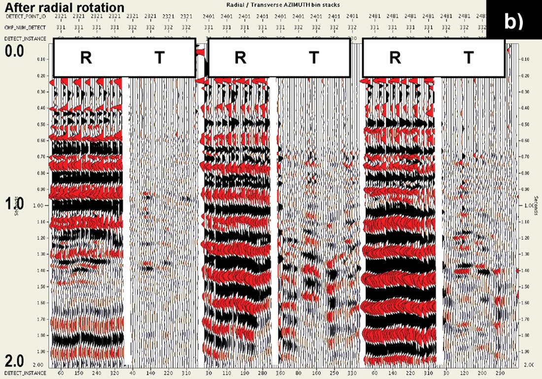
Once satisfied with vector fidelity so that integrity of the shear splitting analysis is assured, attention then focused on deriving full 360° azimuthal analyses on the offset-limited common receiver gathers using sets of raw X, Y component and radial, transverse rotated data. Figure 3(a) shows the X and Y common-azimuth traces for three receiver locations in the southern half of the swath, corresponding to the location of the highest potential for shear splitting. The azimuth traces increase in 10° increments, from 10° to 360°. The same azimuth traces after rotation to radial and transverse are shown in Figure 3(b). Note that most of the energy has transferred to the radial; however, some residual is noted on the transverse which is not all noise. It is also evident that the radial component wavelet response is consistent across the range of azimuths and that below 1.2 s, a sinusoidal pattern is evident, indicating that the PS traveltimes are azimuth dependant; a feature of shear splitting.

Polarization analysis was conducted on the transverse data through detection of polarity flips every 90° change in azimuth using a “snowflakes” time-slice display scheme as described by Bale et al. (2000), and eloquently exploited by Olofsson et al. (2003) and Probert and Kristiansen (2003). In the absence of azimuthal anisotropy, a rotation is not observed and the maximum “snowflake” response aligns with the common acquisition coordinate system. Actual polarization results at different time slices on the southern set of three receiver locations, where the radial sinusoidal effect is clearly evident, are shown in Figure 4. A noticeable rotation in the principal axis of polarization below 1.0 s is clearly visible. It is possible to distinguish between S₁ and S₂ from looking at the earliest arrivals of the radial over the sinusoidal responses at each receiver analysis location. The analysis at receiver location 2161 is shown in Figure 5, where the fast S₁ direction is aligned to 150°/330° (green arrow) with the orthogonal S₂ direction at 60°/240° (blue arrow) corresponding to slower arrival times. The fast orientation of polarization is parallel to the regional normal fault trend and is consistent with the known dominant stress fields within each major fault block.

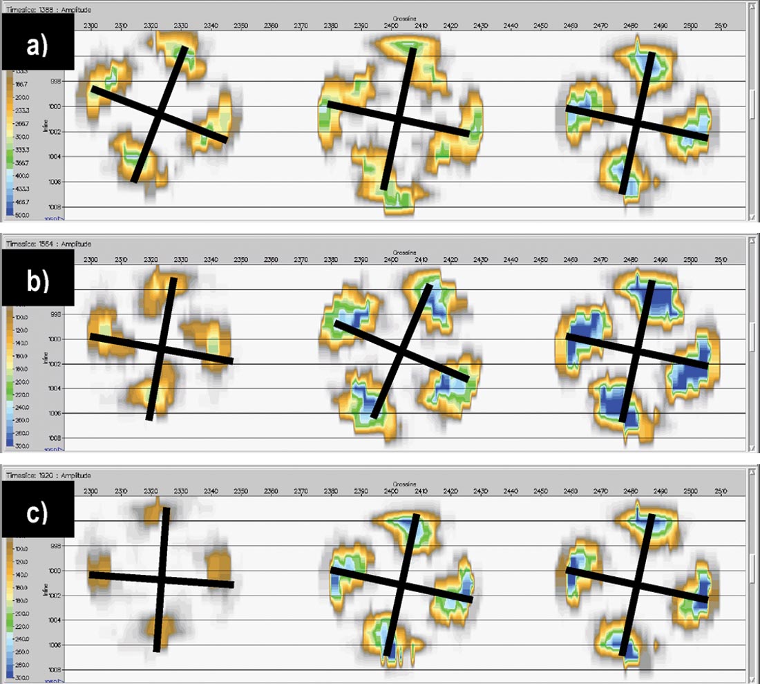
Analysis over the central and northern set of receiver gathers show less residual coherent energy on the transverse and minimal azimuthal variation in velocity. These results are consistent with the transverse stack and indicate less evidence of shear splitting. The polarization analyses at different time slices below 1.0 s reveal a rotation of only a few degrees. Therefore, the strongest evidence of shear splitting, as hinted on the transverse stacks, is constrained to the southern one-third of the swath on the upthrown side of the major fault and is less prevalent elsewhere in the survey.

Anisotropic Prestack Depth Migration

Knowledge of the restrained impact of the azimuthal anisotropy on the PS data provided the necessary confidence to use the preprocessed radial (source–receiver direction) rotated data as input to the PS PrSDM. Special compensation from Alford rotation with layer-stripping correction was not considered essential. For the P-wave, the selected input was the preprocessed PZ data that had been summed using a non-linear PZ combination technique (Moldoveanu, 1996) to deghost receiver-side water-layer multiples.

In the application of PrSDM, a Kirchhoff depth imaging algorithm was selected, that had been routinely adapted to account for PS_v waves with anisotropy and dual surfaces (for the different source and receiver datums from OBC acquisition). Compensation for anisotropy was based on Thomsen’s weak anisotropy relationship for a VTI medium (Thomsen, 1986), using parameters δ and ε. Anisotropy has a greater influence on the description of the velocity for S-wave than with P-wave because the ratio of the square of the vertical Vp/Vs ratio is >> 1 in the expression for the Sv velocity as a function of phase angle, vertical P- and S-wave velocity and Thomsen’s anisotropy parameters.

Of course, the challenge was deriving a valid velocity model to apply in the Kirchhoff PrSDM. That is, a model that produces flat common image point (CIP) gathers across positive and negative offsets, for optimized stack response, and correlates equivalent events on both P- and PSv-wave depth sections at the correct depth confirmed by well data. For this project, the velocity analysis of residual moveout on CIP gathers was performed using a cell-based (gridded) 3D reflection tomography approach. Gridded models allow more flexibility to represent velocity variations that are not easily interpreted from structural dependency in the seismic and are applicable to regions such as the Gulf of Mexico and offshore Trinidad. Due to the inability to perform P- and S-wave tomographic updates simultaneously, the initial priority was to focus on the PZ data and derive a good V(P) model before proceeding to run tomography on the PS data. The work flow that was adopted is summarized as follows:

1. Prestack depth migrate the PZ data with an initial smoothed isotropic P-wave velocity field, derived from the previous time processing.
2. Update isotropic V(P) iteratively from residual velocities using CIP tomography to the flatten gathers.
3. Update V(P) with anisotropy to tie depths at the Pamberi-1 well location deriving both δ and ε to flatten gathers over the depth range of the well.
4. Incorporate the Annie η (Sayers and Johns, 1999) VTI model from the previous time processing to represent the anisotropy below and beyond the proximity of the well. In this instance it was decided to hold δ constant with ε spatially varying.
5. Migrate PZ with the updated anisotropic V(P) model.
6. Migrate PS data anisotropically with the updated anisotropic V(P) and initial smoothed V(S) derived from the anisotropic PSv time processing.
7. Update V(S) model iteratively from residual velocities using CIP tomography to flatten PS gathers.
8. Revise V(S) to register equivalent PZ and PS events in depth. Modify δ and ε as per the original η field.
9. Reiterate with decreasing scalar wavelength using the PS tomography to solve for residual anisotropy ε until solution converges.

The methodology was carried out adopting a top-down approach, prioritizing the shallow section first before progressing deeper.

The CIP tomography automatically picks the residual moveout (RMO) on depth-migrated gathers by identifying the key events based on highest semblance values. It performs various parabolic and linear scans on the identified events and the curve with the maximum semblance is retained at each depth event. An important QC at this stage is to examine residual moveout correction applied to the CIP gather to verify the integrity of the picks and that low-velocity multiple trends or cycle skips are being avoided. Gather conditioning with a mild dip filter was necessary for this dataset. A 3D dip field was created from the depth-converted PrSTM volumes and updated for the final iteration. This dip field together with the RMO picks and initial/previous velocity model, including anisotropy, were then used to solve linear equations relating the RMO change to updates in the velocity model. The changes are linear due to the assumption that raypaths do not change as the velocity model is altered, so depth and velocity have a linear relationship. Consequently, several iterations of CIP tomography are required before an optimum solution, yielding flat gathers, is attained.

For every iteration in the P- and PS_v-wave workflow, the positive and negative offsets were migrated separately to allow determining the residual moveout independently, but solved simultaneously for an update of V(P) in the case of PZ, or V(S) in the case of the PS data.

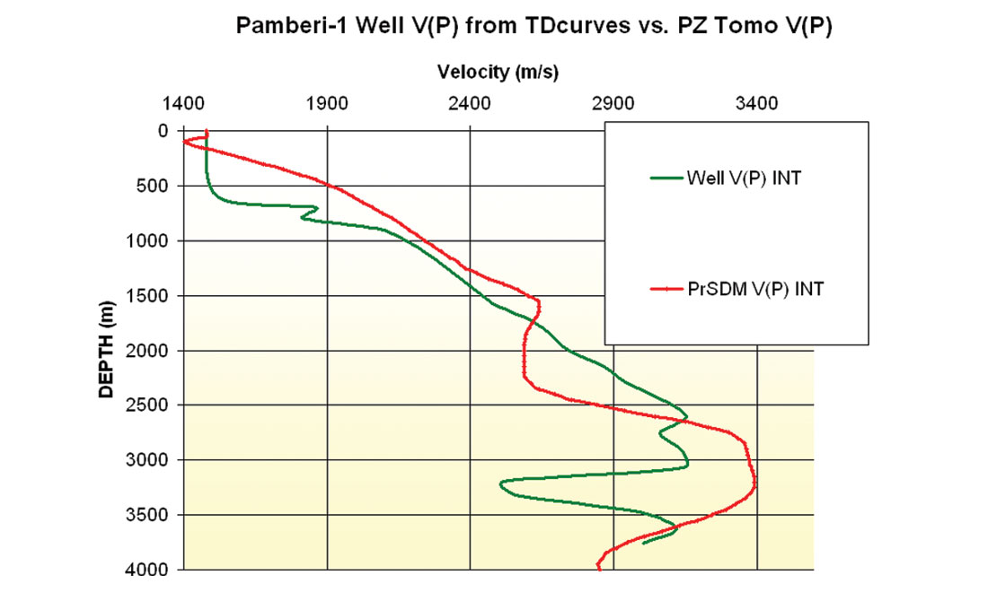
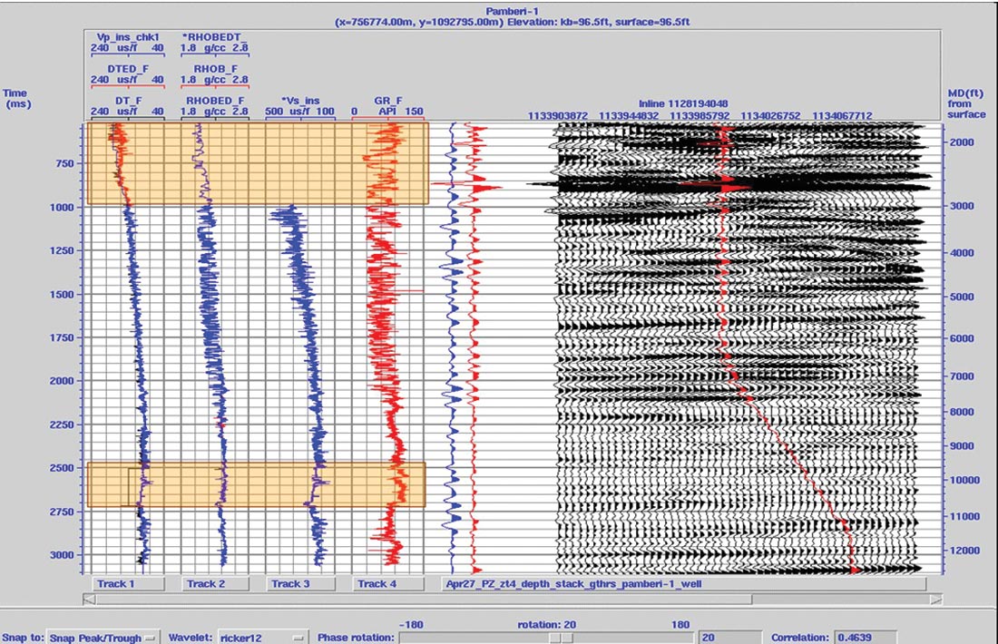
The advantage of having previously performed detailed prestack time migration processing meant that the V(P) and V(S) starting models were reliable and that an initial spatially varying anisotropic field could be incorporated early into the workflow. A display of the PrSDM interval V(P) compared to the checkshot velocity at the Pamberi-1 well is shown in Figure 6, together with the P-wave synthetic. The log contains no shear information, so the well tie was performed on P-wave (PZ) data only. Nevertheless, the log provided a derived 1D set of Thomsen parameters over the 3-km depth interval of the well that could be merged with the 3D VTI model from the time processing. Deeper than 3 km it was initially assumed δ=0 with ε equating simply to the spatially varying η parameter, in accordance with the (Thomsen, 1986) equation:

The anisotropic Thomsen parameters (δ and ε) were further updated after the PZ and PS depth sections were registered to determine the depth discrepancy between the two volumes, as per step 8 in the workflow. For this process to be successful, it is crucial to interpret equivalent horizons on both wave modes. This challenge is compounded by the fact that the shear and acoustic reflectivities are generally different, so the key is to identify common geological features such as faults or channels and map these to a series of horizons. As verified from Zoeppritz forward modeling, the polarity of the PS seismic data in the shallow section must be flipped to achieve optimum wavelet matching of P-P to P-S horizons. The event correlations were originally interpreted on the depth-to-time converted sections to validate the implied interval vertical Vp/Vs ratios. The identified registered horizons were then transferred to the PZ and PS PrSDM sections to deduce the depth discrepancy. A 7% mistie, on average, was measured between the PS and PZ in the 600m to 3400m depth range, requiring a pull-up on the PS section, equivalent to a reduction in V(S).

Discussion of Results

Preliminary prestack analysis of the raw and radial rotated converted-wave data indicated evidence of mild shear splitting from azimuthal anisotropy attributable, in part, to dominant regional stress fields delineated by major fault blocks. The advantage of the detectors exhibiting near-perfect cross-component vector fidelity and orientation facilitated the identification and measurement of principal azimuths of shear-wave polarization on the PS data. It was encouraging to observe that the principal azimuth of polarization agreed closely with known regional lateral stress field orientation for the area. The polarization to S₁ and S₂ was restricted to a rotation of 15° or less from the survey’s natural acquisition orientation, and appeared to have minimal detrimental impact on the final radial rotated PS data quality. From a theoretical standpoint, Alford rotation to principal azimuths of polarization following a layer- stripping approach could most certainly compensate for the differences and yield an incremental improvement, but was outside the scope (and budget) of this project.

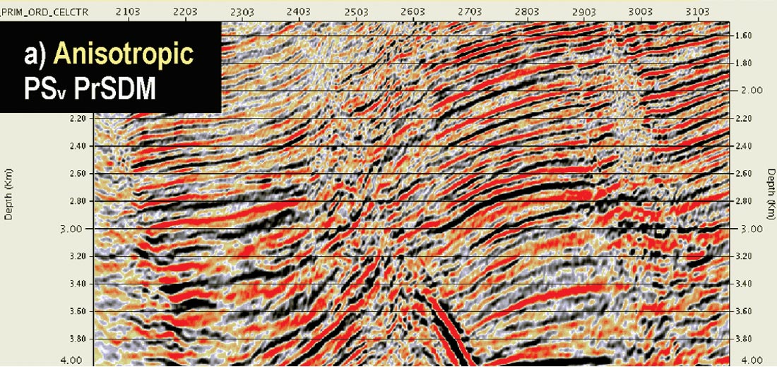
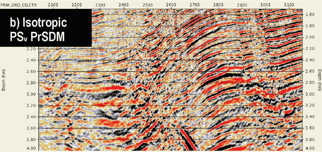
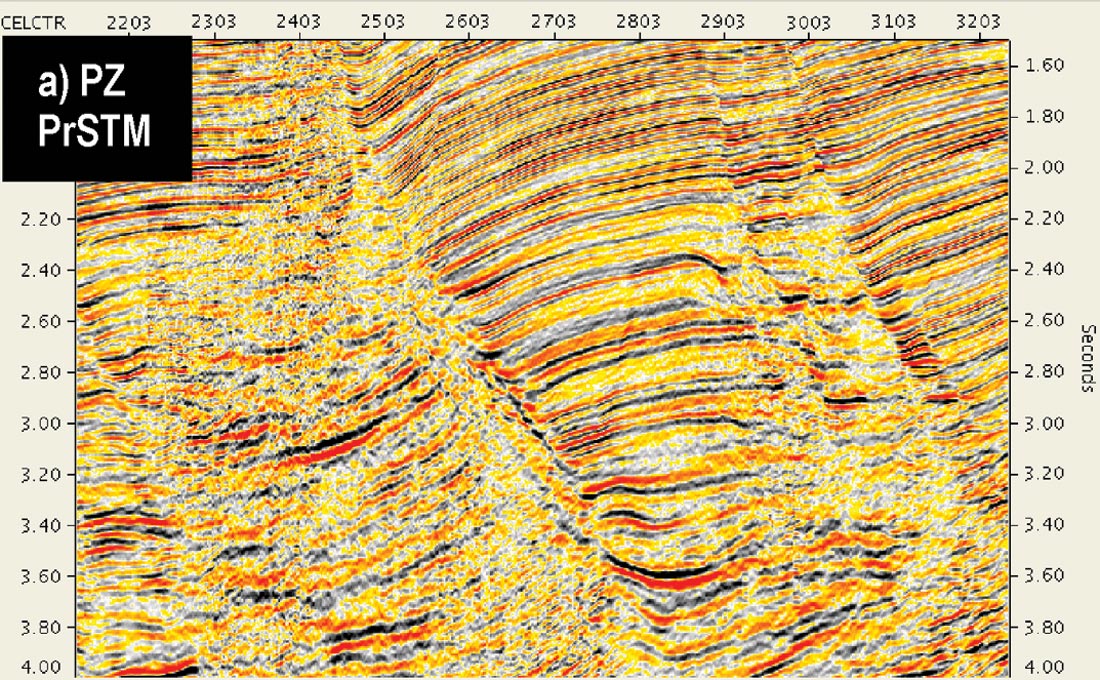
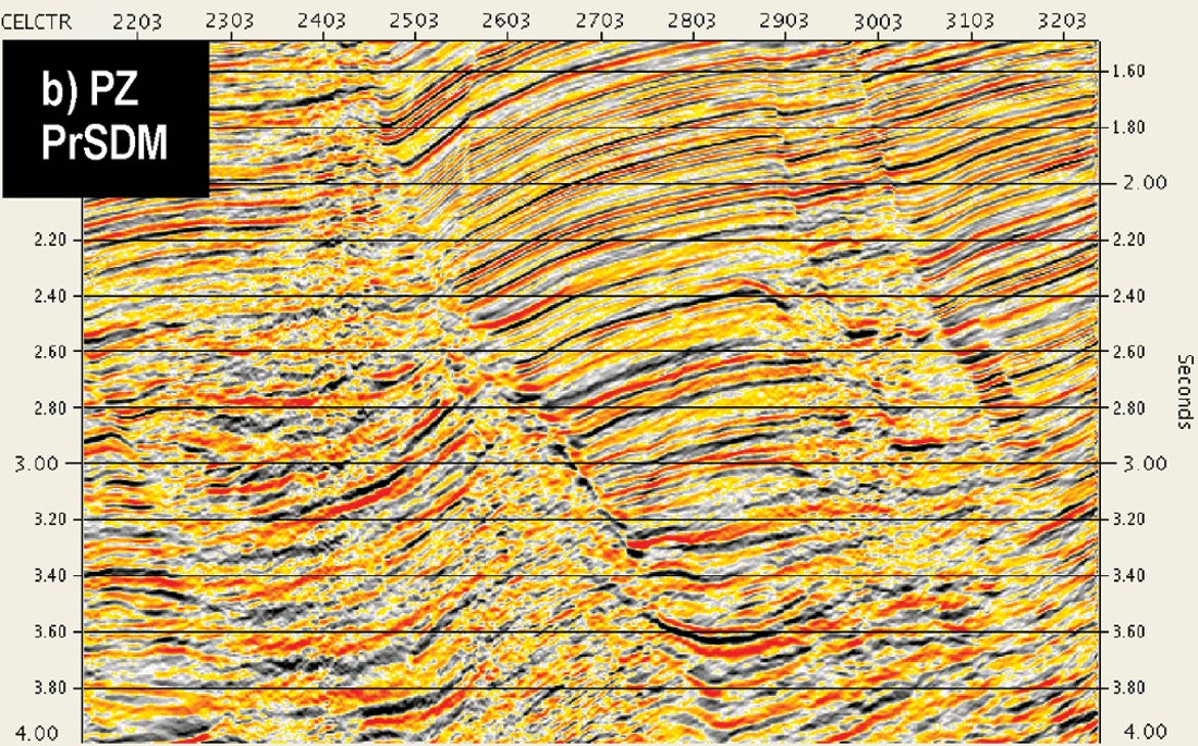
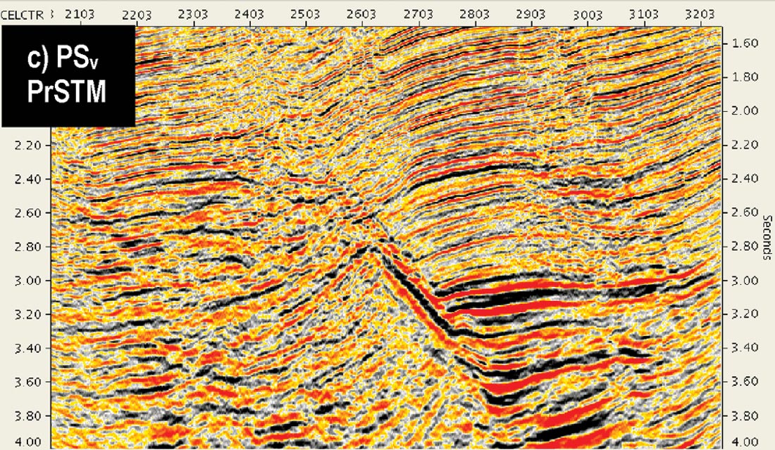
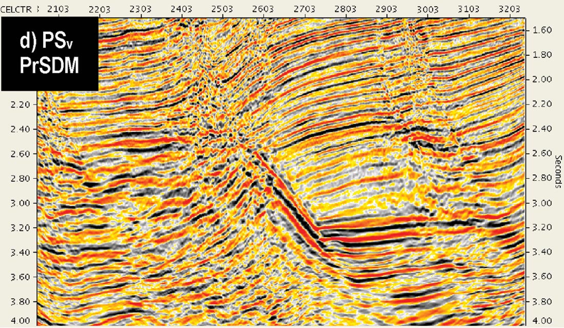
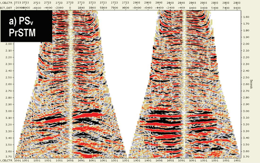
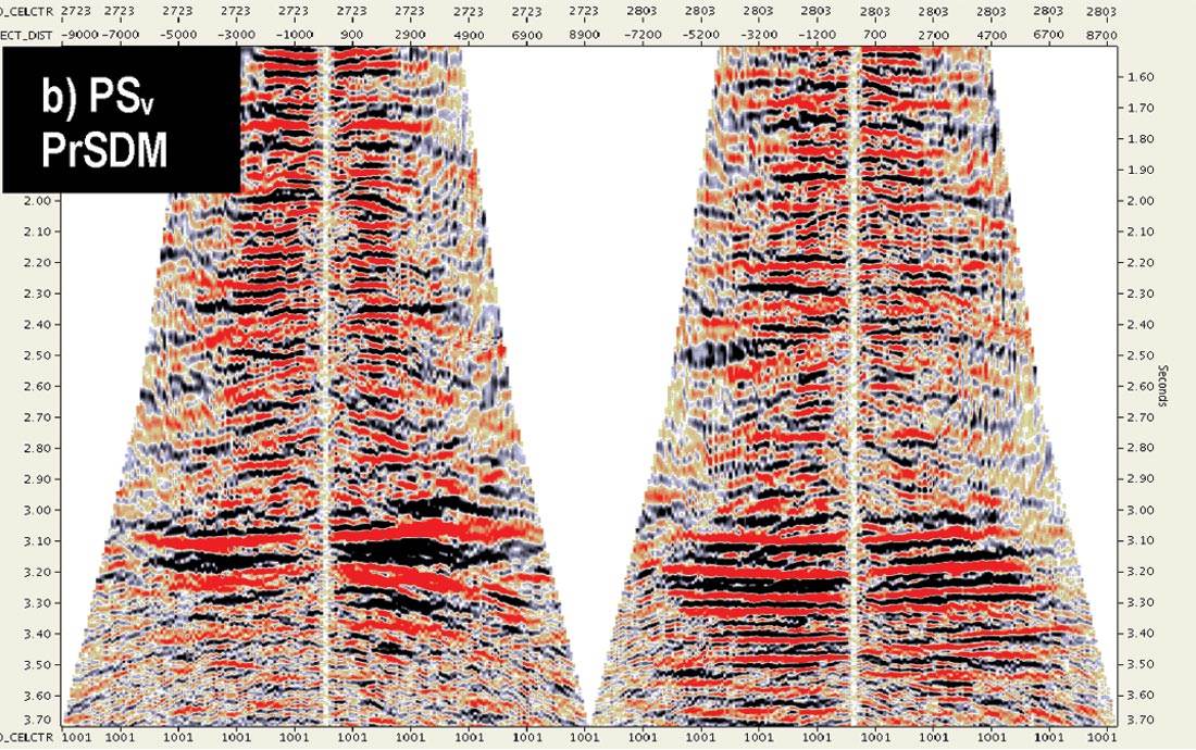
After several iterations of constrained cell-based tomography with progressively smaller scale lengths (smoothing) and the necessary incorporation of anisotropy, the resultant P- and PS_v-wave PrSDM sections are found to exhibit an enhancement in structural detail and continuity, together with improved P-P to P-S_v correlation of target events, across the main fault. The inclusion of anisotropic (VTI) properties from the previous PrSTM (time domain) processing, subsequently updated after well control and detailed P-P to P-S event registration, produced a significant improvement in PS_v imaging, as shown in Figure 7; more so than the impact noted in the P-wave migration. The improvement in structural imaging compared to time-processed PrSTM sections are shown in Figure 8. Furthermore, better flattening of the PS_v depth gathers over the entire positive and negative 10-km offset range, is evident in Figure 9, which is important for future AVO/inversion work in the extraction of rock property attributes. Although raypath asymmetry (Thomsen, 1999) and lateral heterogeneity is causing significant variation in the PS_v reflectivity, structurally there is a better depth consistency match between the positive- and negative-offset PrSDM sections than that noted on the time-processed data, increasing confidence in the PS_v depth interpretation.

Conclusions

In this paper, we demonstrate for the Pamberi area of the Columbus basin of eastern offshore Trinidad, that further to the improvement over the conventional 3D towed-streamer time imaging from 4C anisotropic prestack time migration (Johns et al., 2006), significant enhancement is also possible with anisotropic PrSDM of the P- and PS_v-wave data. Utilizing cell-based tomography for anisotropic velocity modeling, parameterization was further optimized through well control and detailed event registration.

Work currently in progress is now taking advantage of the improved P-P to P-S_v event correlation of the anisotropic depth migrated gathers to quantitatively classify, using additional nearby well control, lithology and rock properties of the target interval from joint prestack inversion.

Despite the acquisition being limited to a single swath, the potential for future work is huge, both in terms of interpretation and processing. The next challenge is to further increase resolution of the P- and PS_v-wave imaging using enhanced preprocessing, advanced migration algorithms, and more interactive anisotropic velocity modeling tools. Any improvement by compensating for the observed azimuthal anisotropy is also a consideration.

Acknowledgements

The authors thank the Trinidadian Ministry of Energy (MOEEI) and EOG Resources for granting permission to publish the results shown in this paper and colleagues at WesternGeco for their processing assistance.