Introduction
The assumption of perfect elasticity of rock materials is made routinely in the geophysical industry and in many, if not most, cases it is an adequate approximation. In making this assumption we ignore a fundamental feature of seismic waves propagating in the real earth which is the absorption of seismic energy by internal friction. Media that dissipate seismic energy are called anelastic. Because absorption increases with frequency, wavefronts are "reshaped" as they propagate. Also, velocities in anelastic media are frequency dependent, leading to apparent wavelet delays.
Our intuitive expectation that anelastic phenomena require a more complicated mathematical formalism is correct; indeed, by comparison the mathematics of perfect elasticity appear almost elegantly simple. Are there any benefits to making use of this increased mathematical complexity in AVO analysis? As it turns out, the presence of anelasticity can either diminish or enhance AVO responses depending on the circumstances, and elastic AVO computations could therefore potentially misinterpret the contributions of intrinsic attenuation as a contrast in velocity and/or density. In addition to the complicating effects of anelasticity, the presence of anisotropy can significantly affect the AVO response. The purpose of this paper is to explore the combined effects of anisotropy and anelasticity on AVO responses through numerical modeling. It is expected that the inclusion of anelasticity into AVO modeling can further reduce uncertainty in AVO analysis.
Theory
The equation of motion for elastic media in Cartesian coordinates is given by (Aki and Richards, 1980)

where u⃗ the particle displacement vector and λ and μ are the Lame parameters of the elastic medium. Anelasticity can be modelled by invoking the linear theory of viscoelasticity (Krebes, 1980, Chapter 2). In this theory, an anelastic material is said to have "memory" or, in other words, the properties of the medium at a given time depend on the history of the stress applied up to that time. The effect of absorption is generally accounted for by the quality factor Q. Most researchers consider Q to be constant in the range of seismic frequencies.
The stress-strain relation for a homogeneous isotropic linear viscoelastic medium is given by (Krebes, 1980, Chapter 2).
where
σ is the stress tensor,
δ is the Kroeneker delta,
e is the strain tensor and
λ(t), μ(t) are time dependent Lame parameters which describe the "memory" of the anelastic medium. Substituting this stress - strain relation into the equation of motion (1) yields the equation of motion for anelastic media below

where the symbol * denotes Stieltjes convolution.
It can be shown (Krebes, 1980, Chapter 2) that, as a mathematical consequence of equation (3), P-wave velocities and S-wave velocities in anelastic media are frequency-dependent.
P-wave propagation properties of anelastic materials can be described by only two parameters, for example Q and phase velocity at an arbitrary reference frequency (Kjartansson, 1979). Frequency dependent velocity v(f) as a function of both Q and reference velocity V(fref ) is given by
See for example Kjartansson (1979) or Aki and Richards (1980). The definition of the quality factor Q introduces amplitude decay per wave length given by

In addition to several theoretical proofs for equation (4) there also exists experimental evidence.
Equations (4) and (5) are commonly combined, leading to anelastic velocities that are frequency-dependent and complex. Propagation and attenuation vectors are then derived from complex horizontal wave numbers which are caused by these complex velocities. Fig. (1) shows a family of v(f) curves computed with equation (4), where Q ranges from 10 to 100. The reference frequency fref was arbitrarily set to 30Hz. Note that velocity logs are usually acquired with a measurement frequency much higher than that. For Q-factors much above a value of 100, the curves would be essentially flat in the seismic range of 10 to 100 Hz.
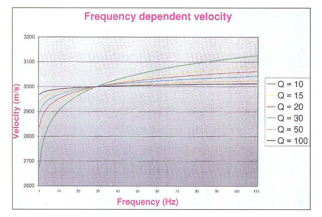
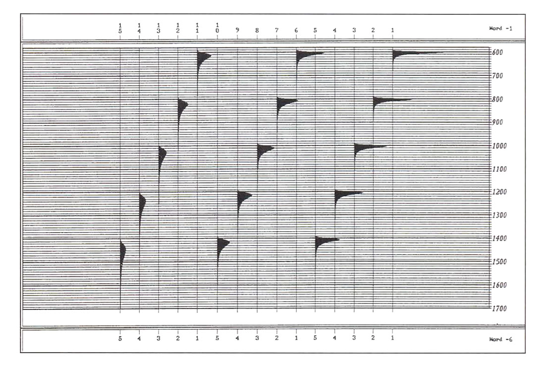
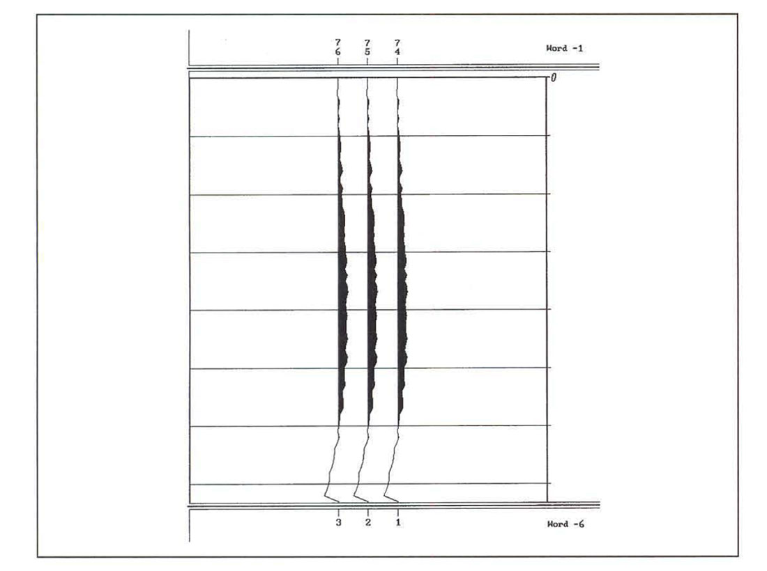
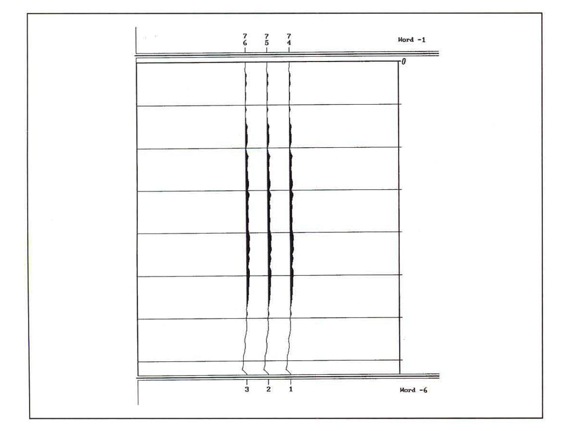
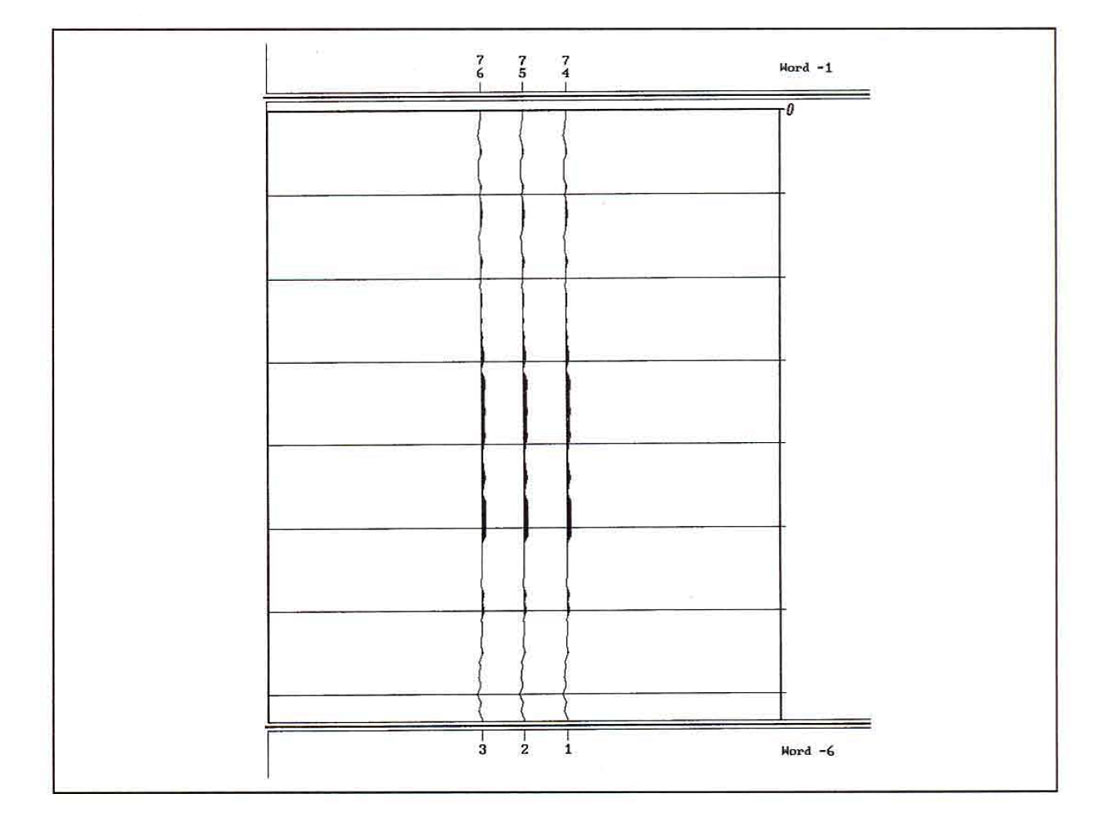
Fig. (2) was computed with equations (4) and (5), assuming v(125Hz) = 3000m/sec and Q=25, 50, 100 (from left to right) for depths from 1800m to 4200 m (step 600m) given an impulsive plane wave source at the surface. Wavelet spread and attenuation shown agree with the results obtained by H. Kolsky (1956) from experiments carried out on rods of viscoelastic solids.
The question as to whether or not it is correct to apply the linear theory of viscoelasticity to anelastic rocks is investigated by E. Kjartansson (1979). He states that the magnitudes of both propagation velocity and Q are independent of the amplitude of the passing seismic wavefield at strains less than. This strongly suggests that the material response at these strain regimes is dominated by linear effects and that nonlinear effects can only be significant very near the source. In his conclusions Kjartansson also remarks that it is likely that Q is weakly dependent on frequency.
AVO in anelastic isotropic media
What changes can be expected for AVO in anelastic media? For finite Q, attenuation of wave fronts increases with distance travelled and therefore amplitudes are diminished with increasing offset. Depending on the sign of the AVO gradient, this could either reduce or enhance an elastic AVO-response (Carcione et al, 1998).
Before proceeding to compute AVO-responses we make a conjecture. By inspection of AVO-responses derived utilizing the propagation/attenuation vector approach, we observe that amplitude and phase can change drastically near and beyond critical angles. In the region of pre-critical angles amplitudes are well behaved and phase angles are near zero.
We therefore assume that, for pre-critical raypaths and Q larger than say 10, at a given frequency, travel times can be computed with sufficient accuracy from equation (4) and Snell's law alone, and amplitude decay due to anelastic absorption of seismic energy can be computed with sufficient accuracy from equation (5) alone. Neither mathematical proof nor a counter example for this conjecture could be found up to the time of writing.
Two more steps are required before AVO-response computations can proceed. Firstly, the geometrical spreading equation (Ursin (1990), Krebes and Slawinski (1991))
is introduced to account for amplitude decay caused by wave front spreading alone. Secondly, in order to compute reflection and transmission coefficients, the Zoeppritz equations are employed. Thus, errors due to approximating the plane wave Zoeppritz equations are avoided, but it must be assumed that the shallowest reflector is at least several wavelengths below the source point.
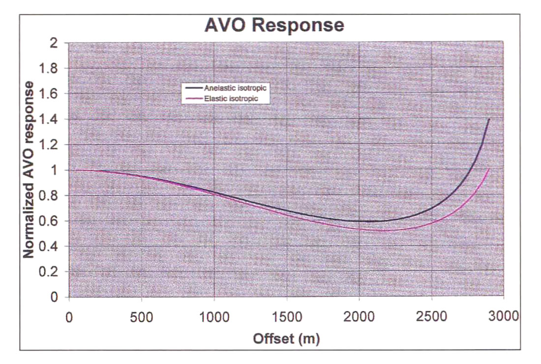
The earth model shown in Table 1 (adapted from Krebes, 1998) is used to compute the AVO-response given in Fig.3, Thomsen parameters δ and ε are set to zero for an isotropic response and zero offset amplitudes are normalized to unity. H is layer thickness, α and Β are P-wave velocity and S-wave velocity, respectively. The elastic AVO-response shown in Fig. 3 for comparison was computed with Qp and Qs, set to a very large (but finite) value. Anelasticity does in fact enhance AVO-response for this earth model when compared to the elastic case.
| Layer | 1 | 2 | 3 |
| Table 01 | |||
| H(km) | 1 | 1 | 1 |
| α(km/s) | 1.8 | 2.5 | 3.6 |
| Β(km /s) | 0.9 | 1.4 | 2.1 |
| ρ(kg/m3) | 2000 | 2100 | 2200 |
| Qp | 25 | 30 | 45 |
| QS | 12 | 17 | 20 |
| δ | 0.1 | 0.1 | 0.1 |
| ε | 0.1 | 0.1 | 0.1 |
AVO in anelastic media with velocity-anisotropy and isotropic Q
What would be the AVO-response of media that are both anelastic and anisotropic? Anisotropy means that velocities depend on direction of wavefront travel, in addition to frequency dependence of velocities introduced by anelasticity. Similar to the isotropic situation, anelasticity will diminish amplitudes with increasing offset, which could either reduce or enhance elastic anisotropic AVO gradients. This observation is confirmed by the results of Carcione et al. (1998).
The anelastic anisotropic AVO-responses shown in Fig. 4 are computed for the earth model given in Table 1, and VTI-type anisotropy is assumed. Anisotropic P-wave AVO behavior is usually approximated by adding an anisotropic correction term to the isotropic reflection coefficient (Tsvankin, 1996); however for the earth model given in Table 1 this correction term is zero because Thomsen parameters do not change across interfaces. Under this simplifying assumption of spatially invariant Thomsen parameters, the only change required to the AVO computation algorithm when compared to the isotropic case is the introduction of an isotropic raytracer.

Note that Table 1 shows a special kind of anisotropy (elliptical), but reducing δ to zero or increasing ε to unity changes the AVO response very little. The introduction of VTI-type anisotropy in addition to anelasticity serves to further enhance the AVO response for this earth model (Table 1).
AVO in anelastic media with velocity-anisotropy and Q-anisotropy
In addition to velocity-anisotropy, there is also evidence for Q-anisotropy (Waters (1987), Yin (1993)) which further complicates AVO behaviour. K. Waters (1987) showed empirically that compressional- wave Q is approximately proportional to the square of compressional-wave velocity or
For anisotropic media, the distinction between group velocity (or ray velocity) and phase velocity (or wavefront velocity) must be made. The phase velocity v(θ in terms of Thomsen parameters is given by Tsvankin (1996) as
α0 is the vertical P-wave velocity and
β0 is the vertical S-wave velocity
The relationship between phase velocity v(θ) velocity V(ϕ) is given by J.G. Berryman (1979) as
The presence of Q-anisotropy will affect the determination of the group velocity, which in turn governs the speed at which wavefronts propagate in anisotropic media.
To see this, note that the second term on the RHS of equation (9) is not only controlled by the θ-dependence of the anisotropic velocity but, through equations (4) and (7), also by the θ-dependence of the anisotropic Q. The second Ava curve shown in FigA is computed for the earth model given in Table 1, assuming VTI-type velocity-anisotropy and Q-anisotropy. Compared to the isotropicQ case, the introduction of Q-anisotropy in addition to VTI-type velocity-anisotropy enhances the AVa -response yet again for the earth model of Table 1.
J.P. Blangy (1994) considers elastic and anelastic VTI shales overlying isotropic sands (gas-sands and water-sands) and finds that in all his cases, the effect of anisotropy on Ava is enhanced by anelasticity. He also observes that the impact of Q-anisotropy on AVa -responses can be of the same order as that of velocityanisotropy: Assuming the direction of slowest velocity in a TI-medium and the direction of the greates t intrinsic attenuation are the same (which is a reasonable assumption for most cases encountered in exploration situations), he states that the effects of velocity-anisotropy and Q-anisotropy are expected to add constructively.
Fitting a Dix-approximation hyperbola to anelastic moveout
From equation (4) it is apparent that, for anelastic media, the velocity is different for each frequency point; the smaller Q, the larger the difference. Fitting a Dix-approxirnation hyperbola to an anelastic moveout curve during routine velocity analysis results in one velocity estimate only; how does this estimate compare to the range of frequency dependent velocities? A simple earth model is constructed in order to compute some actual numbers. A single reflector in an isotropic homogeneous anelastic medium is located at 1800m depth. Veloci ty is 3000 m / sec at a reference frequency of 125 Hz. Reflectivity is set to unity for all offsets, and geometrical spreading is not included in this model.
Table 2 shows the result of the least square error fit velocity analysis.
| Q | 25 | 50 | 100 |
| Table 02 | |||
| Vstack(m/ s) | 2885.7 | 2957.1 | 2985.2 |
The fact that the best fit velocity decreases with decreasing Q is not surprising: the lower the Q, the more the higher frequencies are attenuated and the remaining lower frequencies travel at slower velocities. A residual moveout comparison is shown in Fig. 5 and interestingly, there are signs of non-hyperbolic moveout for the lower Q-factors. This result is reminiscent of anisotropy, but the earth model employed here is isotropic and anelastic. Further study is required in order to confirm this unexpected result.
Summary and conclusions
Anelastic media are said to have "memory" and velocities are frequency dependent. Seismic energy is absorbed and wavelets spread in proportion to distance traveled. The linear theory of viscoelasticity can be used to model seismic anelasticity, whereby a frequency independent Q completely describes attenuation of seismic waves.
In media that are both anisotropic and anelastic, velocities depend on direction and on frequency. Anisotropic AVa-responses can either be enhanced or diminished by the presence of anelasticity, depending on the circumstances. In addition to velocity- anisotropy, there is also evidence for Q-anisotropy. The impact of Q-anisotropy on AVO-responses can be of the same order as that of velocity-anisotropy, and the two effects are expected to add constructively in most exploration situations.
We have seen that anelasticity and anisotropy can modify AVOresponses. If these factors are not considered, a misinterpretation of AVO trends could result.

Acknowledgements
Thank you to O. Kuhn and M. Perz for their help in preparing this article.


Join the Conversation
Interested in starting, or contributing to a conversation about an article or issue of the RECORDER? Join our CSEG LinkedIn Group.
Share This Article