An integrated strategy: constrained tomography inversion of multi-type data for near surface velocity model building

After analyzing the theory assumptions and the pros and cons of three methods in near surface model building, which have been widely used in data processing, the three of us all agree that an “Integrated Strategy”, based on constrained first arrival tomography inversion, should be introduced as described in this paper. Compared with other data processing methods in near surface model building, the new method, using multi-type data in a constrained tomography inversion, can achieve a higher resolution near surface model for both geological data and geophysical data.

Introduction

A complex near surface can severely degrade the acquisition of land seismic data and negatively impact the subsequent processing. In the past few decades, static correction is still a “bottle neck” in land data processing which distorts seismic image quality. To address this issue, a lot of effort has been made in order to build up an accurate near-surface velocity model. Currently, three methods for building the near surface model are used. The first one is based on the field measurements for the shallow low velocity zone, such as small detailed or shallow refraction and up-hole data. The accuracy of the near-surface velocity model largely depends on the sampling density of the control points and the data quality at each control point in the field survey.

The second method is based on refraction propagation theory with an assumption that the geology model consists of “layered” media with constant velocity in each layer, such as the time-delay method, or the general reciprocity method. Generally, this kind of technology works well in areas where the near surface model is relatively simple. However, for complex areas such as mountain and desert areas, this method will break down due to the strong lateral velocity variation and the rapid change in the layer thickness. Therefore, it is difficult to obtain the desired static correction results. These two methods may also generate false structures by creating a medium and long wavelength static correction problem.

The third method is first arrival tomography inversion. It not only needs refraction arrivals, it also needs direct-wave arrivals and turning-wave arrivals. In its implementation, the near-surface model is parameterized by grid cells, each cell having a constant velocity. The final velocity model can be inverted by iteratively solving linear equations using an optimization algorithm. Theoretically, tomographic inversion is able to deal with complex near surface velocity distribution with strong lateral velocity variation; however the results are also impacted by the geometry and picking quality. Additional errors may be induced in cases where there is a limited acquisition aperture, a lack of near offset traces, or a sparsity of picked first arrivals.

Based on the above discussion, different types of data carry different information for velocity estimation. The detailed or shallow refraction and up-hole data are able to provide a shallow velocity model with high accuracy at the sparsely measured locations. These measurements are useful supplements for tomography inversion to mitigate the errors caused by the lack of near offset traces and the shot deviation from the receiver line in 2D cases. Simply using one kind of data may not adequately describe the near surface heterogeneities. Therefore, it is necessary to develop a new strategy to integrate different types of data for near-surface velocity inversion. The constrained tomography inversion proposed in this paper takes advantage of the integration of seismic first arrivals, up-hole times, and detailed or shallow refraction survey information in order to help reduce artifacts and produce a more accurate near-surface model for static correction processing.

Constrained Tomography inversion

The constrained tomographic inversion equations can be expressed as follows,

Where A, ΔS and ΔT, are Jacob matrix constructed by a ray tracing algorithm, slowness and travel time residual respectively; M is the number of rays and N is the number of cells. Matrix C in equation (2) can be obtained using equation (3),

where Si is the slowness in the i^th cell. When the cell is located within the shallow details of the velocity model and in the up-hole-velocity measurement zone, there will be no update during iteration.

The final joint inversion equation can be expressed as:

Where, B (M + L) × N dimensional matrix

And where

The objective functions for Lagrange constrained optimization is:

The optimal solution will be achieved by iteratively solving the above equations by LSQT. The lambda in equation (5) is a regularization parameter. A bigger value of lambda means a stronger constraint applied to inversion. When λ = 0, the constrained tomography is reduced to a conventional non-constraint tomography inversion.

Application Example

The constrained tomography inversion method is applied to a 2D line from west China. Figure 1 depicts the result from the conventional non-constraint tomography inversion. There are five up-hole control points on the line. The height of the green bar in Figure 1 shows the depth and position of each up-hole. The black solid line represents the high velocity interface. It can be seen that no up-holes reach the high velocity interface. The non-constraint tomography inversion result is shown again in Figure 2, overlaid with the velocity of the five up-holes. It is obvious that the velocity in the very shallow part does not tie well with the velocity values from up-holes. Figure 3 shows the velocity model from the constrained first arrival tomography inversion that uses the right four up-hole control points. It can be seen that the constrained tomography inversion remarkably improved the near surface velocity model accuracy. More importantly, the new inversion results provides more low velocity information in the absence of up-holes and the results match well with the geologic situation.

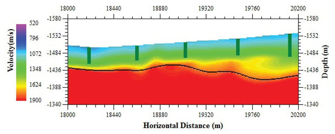
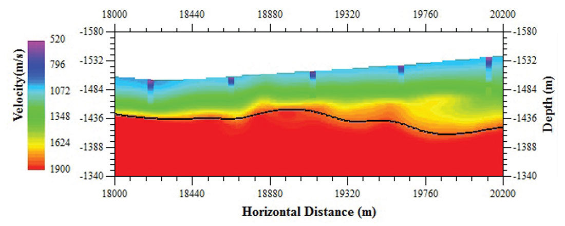
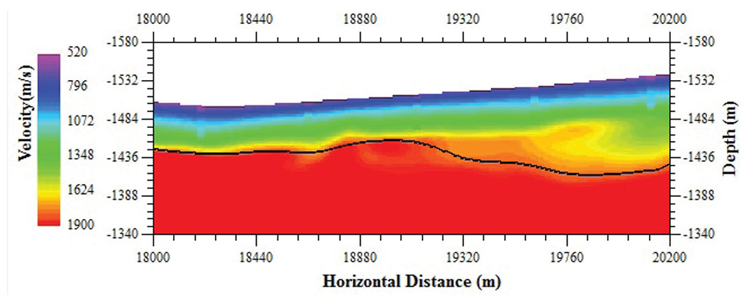
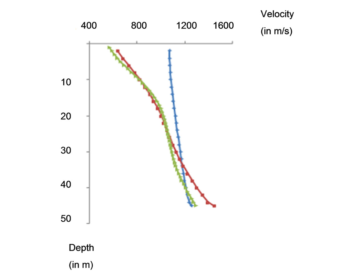
Figure 4 compares the velocity models at the left up-hole location which was not used to constrain the inversion. The blue, red and green lines represent the velocity result from the non-constraint tomography inversion, constraint tomography inversion and the up-hole data, respectively. It is observed that the constraint tomography inversion result (in red) matches the up-hole velocity data profile (in green) with high quality. The analysis using the average velocity within the bottom of the up-hole profile and the inversion results demonstrates that the constrained inversion improves the velocity model with an accuracy of 96% compared to the conventional tomography inversion with an accuracy of 82% in this test example.

Conclusions

The proposed constrained tomography inversion takes advantage of of up-hole control points, detailed or shallow refraction, and seismic data to mitigate the solution ambiguity and improve the accuracy in first arrival tomography inversion. The application of this method to field data sets demonstrated that this method proves to be effective in building an accurate near surface velocity model and is capable of reducing the artifacts.

Acknowledgements

The authors would like to thank Talimu Oilfield of CNPC for permission to show the field data.