A Robust Joint Inversion Algorithm for Rock Property Estimation

Introduction

In the last decade or so, there has been increased interest in prestack inversion. This is because prestack inversion can extract not only compressive information but also estimates of shear information about a rock. The shear wave information is obtained from the variation of reflection coefficients with source-receiver spacing in multi-offset seismic data (i.e., AVO). Both P and S wave velocities of rocks are required to detect the fluid content within reservoirs. This is due to the fact that P waves are sensitive to changes in pore fluid and may travel at drastically reduced velocity, while S waves do not see the fluids within the pore spaces of the rock. These different behaviours of P-waves and S-waves when fluid change in the pore spaces make prestack inversion useful as a direct hydrocarbon indicator in clastic rocks.

In this article, I describe a procedure as how zero-offset P and S-wave reflectivity series are extracted from NMO corrected CMP gathers, and then go on to demonstrate a robust joint inversion approach to simultaneously estimate acoustic and shear impedance from P and S reflectivity series. The inverted acoustic and shear impedance are combined to derive rock properties such as Vs/Vp, Poisson's ratio, Poisson reflectivity and Lamé's constants, which then can be used to estimate reservoir parameters such as lithology, porosity and fluid content. Burianyk (2000) has given a simplified review of the general procedure for estimating rock properties from seismic data.

Amplitude variation with offset (AVO)

The Zoeppritz equations describe the relations of incident, reflected and transmitted longitudinal waves and shear waves on both sides of an interface. For analysis of P-wave reflections we only need an equation which relates reflected P-wave amplitudes to incident P-wave amplitudes as a function of the angle of incidence. In practice, many researchers have simplified Zoeppritz equations. Recently Fatti et al. (1994) re-arranged the Zoeppritz equations, expressing the offset-dependent P-wave reflection coefficients as a function of zero-offset P-wave reflectivity and

where I_p = V_pρ is acoustic impedance, I_s = V_sρ is shear impedance, ΔI_p/2I_p is the zero-offset P-wave reflectivity and ΔI_s/2I_s is zero-offset S-wave reflectivity, and θ is the average angle of incidence. The Fatti formulation makes no limiting assumptions about V_s/V_p or density, and are valid for higher incident angles than many other similar approximations. To extract P- and S wave reflectivities (ΔI_p/2I_p and ΔI_s/2I_s), one needs to apply the least squares method to fit equation (1) to the P-wave reflection amplitudes from real data CMP gathers (Smith and Gidlow 1987). These two reflection coefficients have been combined to obtain fluid factor traces that can indicate the presence of gas (Fatti et al. 1994); Gas sandstone in a clastic sequence gives rise to high fluid factor amplitudes, while all other reflections have low amplitudes.

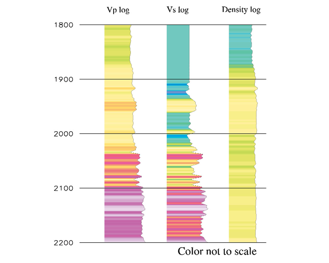
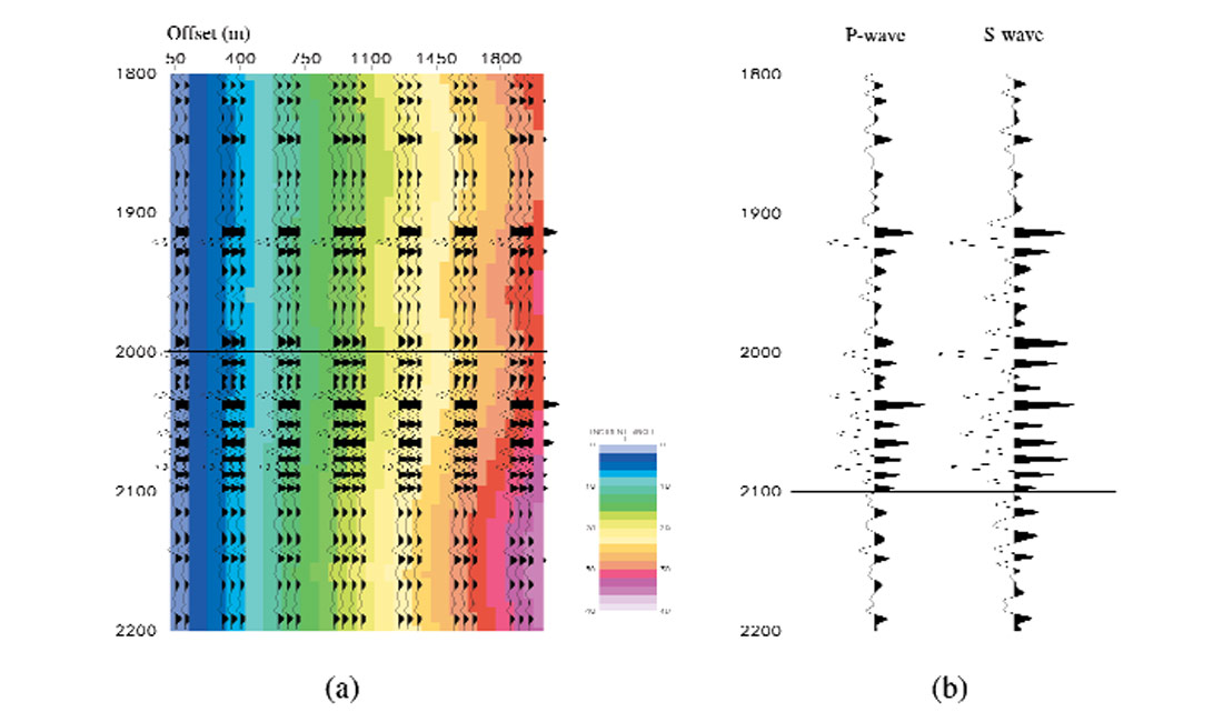
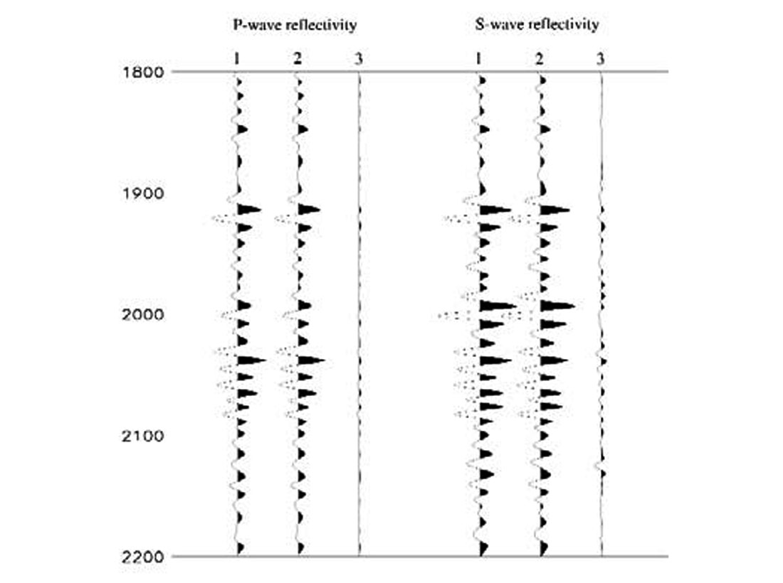
To illustrate how the AVO extraction is performed, I generate a synthetic seismic gather using the Zeoppritz equations. Three logs (P-wave velocity, Vp, S-wave velocity, Vs and density, ρ (see Figure 1) are required by the Zoeppritz equations to generate offset-dependent reflection coefficients. A Ricker wavelet is used to convolve with reflection coefficients, simulating band-limited seismic data (Figure 2a). Now I run the least squares fitting program to extract reflectivities from the CMP gather and results are shown in Figure 2b. It can be seen that we can extract shear-wave estimates from P-wave data without recording shear waves. Note that both P and S seismic traces have the same two-way travel time to a specific reflector controlled by the P-wave velocity.

To understand rock properties for reservoir characterisation, these two reflectivity data must be inverted to reveal the geology of layers rather than the changes at layer boundaries. Rock properties such as velocities, Poisson's ratio and acoustic and shear impedance are more readily tied to well logs, and more directly related to reservoir properties. They are often a direct hydrocarbon indicator and also useful for mapping fluids within the reservoir and improving volumetric estimation.

A joint inversion scheme

Seismic inversion is the calculation of the earth's structure and physical parameters from some sets of observed seismic data. Many inversion algorithms now exist in industry. In the last decade or so, there has been increased interest in model-driven inversion. This algorithm is based on forwarding modelling of seismic data. Synthetic seismograms are generated from an initial subsurface model and compared to the real seismic data; the model is modified and the synthetic data is updated and compared to the real data again. If after many iterations no further improvement is achieved, the updated model is taken to be the inversion result. A priori information is usually incorporated in order to improve the uniqueness of the output. The above inversion process can also be described within an optimisation framework. i.e., one needs to find a global minimum of an multi-variable objective function by means of an optimisation procedure. Once the global minimum is found, the corresponding model parameters are the resultant earth model. Below, I describe a robust joint inversion scheme and show how both acoustic (P) and shear (S) impedance are inverted simultaneously using an optimisation approach.

An optimisation procedure requires a misfit criterion (objective function) to evaluate the quality of each trial model. An objective function may contain multiple terms allowing different types of constraints to be built into the model. For the method described here, I use an L1-norm error function, which is the least absolute deviation between the observed and modelled seismic trace. An a priori impedance constraint is built in, which forces the solution to be close to the low frequency impedance trend. An a priori Vs/Vp ( = Is/Ip) constraint is also added to guide the search to follow the

where S_pⁱ_obs, S_si_obs are P and S reflectivity traces derived from observed seismic gathers; S_pi_mod, S_si_mod are synthetic P and S reflectivity traces; I_pⁱ_pri, I_sⁱ_pri are P and S impedance macro models; I_pⁱ_mod, I_sⁱ_mod are modelled P and S impedance; W₁,W₂,W₃ are weights applied to the above three terms, and n is number of samples in the seismic inversion window. Note that while the number of terms in the above summations is n, the exact number of parameters solved the global optimisation is 2n; the parameter vector consists of n P-impedance samples followed by n S-impedance samples.

To find a global minimum of the objective function, I use a global optimisation algorithm called simulated annealing. Simulated annealing mimics the physical process by which a crystal forms by slow cooling of a melt until the global minimum energy state is reached. It explores the objective function's entire surface and tries to optimise the function while moving both uphill and downhill. Within the annealing procedure, a random point in the model space is selected and the energy or misfit is calculated. The new model is accepted unconditionally if the energy associated with the new point f' is lower (Δf = f'-f < 0). If the new point has a higher misfit (Δf > 0), then it is accepted with the probability p = exp(Δf/T) where T is a control parameter called the acceptance temperature. This acceptance criterion is known as the Metropolis rule (Metropolis et al. 1953). The generation acceptance process is repeated several times at a fixed temperature. Then the temperature is lowered following a cooling schedule and the process is repeated. The algorithm is stopped when the error does not change after a sufficient number of trials. Since the probability of accepting a step in an uphill direction is always greater than zero, the algorithm can climb out of a local minimum (Ma, 2001).

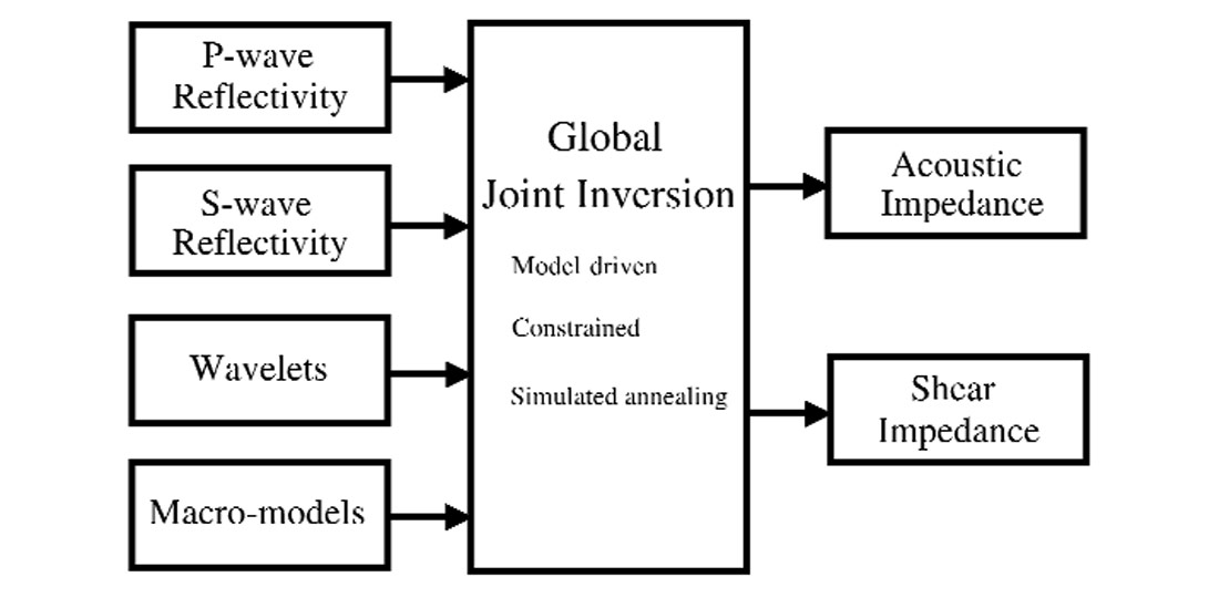
To model synthetic P and S-wave seismic data, I use a convolutional model, i.e. a seismic trace is considered as the convolution of reflection coefficients with a wavelet. Within the joint inversion scheme, synthetic P- and S- seismic traces are generated separately and compared with observations to form a measure of the misfit. The inversion procedure requires many thousands of forward modelling steps to converge on an acceptable solution. The joint inversion algorithm takes as input P- and S-seismic, and macro P- and S- impedance models and a wavelet. It outputs both acoustic (Ip) and shear (Is) impedance models (Figure 3).

Synthetic data example

One set of P-wave velocity, V_p, S-wave velocity, V_s, and density, ρ logs defines elastic properties for a horizontally layered and isotropic 1-D medium (Figure 1). I use these 3 logs to generate a synthetic seismic CMP gather. The gather, superposed on the incident angle, is shown in Figure 2a. The P- and S-wave reflectivities are extracted using the Fatti's AVO equation and are shown in Figure 2b. The objective of this test is see how well acoustic and shear impedance can be inverted, given reflectivity data, macro-impedance models and a wavelet.

The simulated annealing algorithm begins by calculating the objective function using the initial model parameters. After that, one parameter is perturbed randomly within a specified range and the objective function evaluated again. This move is either accepted or rejected according to the Metropolis criteria. The remaining parameters are perturbed in turn and evaluated for the acceptance and rejection in the same manner. The process is repeated until a sufficient agreement between the observed and the synthetic data is achieved. The outputs are the optimised acoustic and shear impedance values. Figure 4 shows the inverted P and S impedance along with true impedance logs and macro-impedance models. It can be seen that the match between the log and inversion is very good. To assist quality control, the synthetic seismic traces calculated using the inverted impedance profile have been plotted along with the "observed values". They indicate that most of the energy in the 'observed' traces have been inverted (Figure 5).

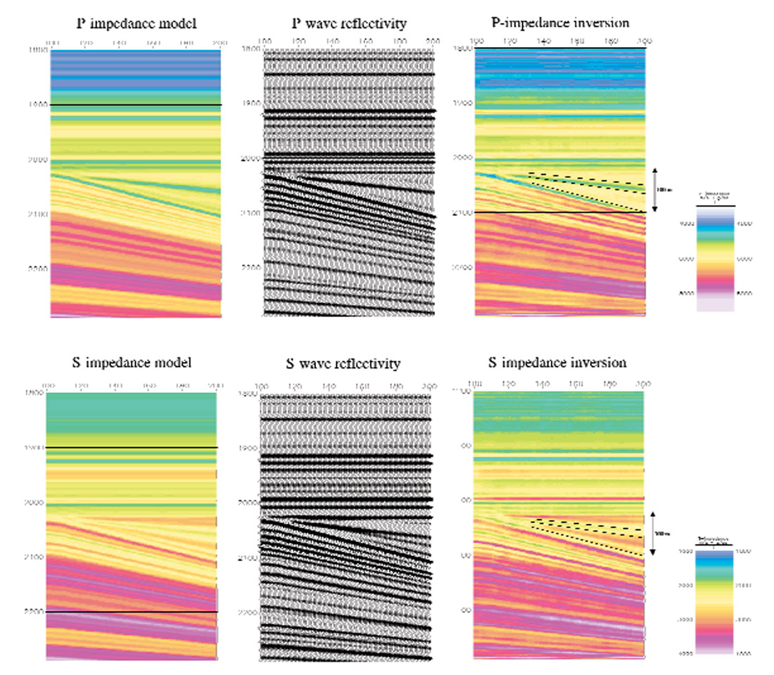
In order to examine the resolution of inverted impedances, I create a sand wedge model in which the thickness of sand varies from 0 to 100 m. The layer properties of the model are taken from the same logs (see Figure 1). Again, synthetic seismic gathers are generated using the Zoeppritz equations, and P and S reflectivities extracted through fitting the Fatti's AVO equation to the gathers. The jointly inverted acoustic and shear impedances are shown in Figure 6a and 6b. It can be seen that the resolution and trace to trace continuity are high, demonstrating the stability of the method.

Field data example

The prestack seismic data presented here is from a North Sea 3D survey. True-amplitude processing including pre-stack time migration was performed and normal moveout corrections carried out. There were three wells in the area, where P-wave and density logs were available. S-wave logs were derived from the Vs and Vp relationship, obtained from nearby wells outside this survey area. These logs were used along with seismic horizons to construct macro-velocity and impedance models. A wavelet was estimated at one well location and used for forward modelling.

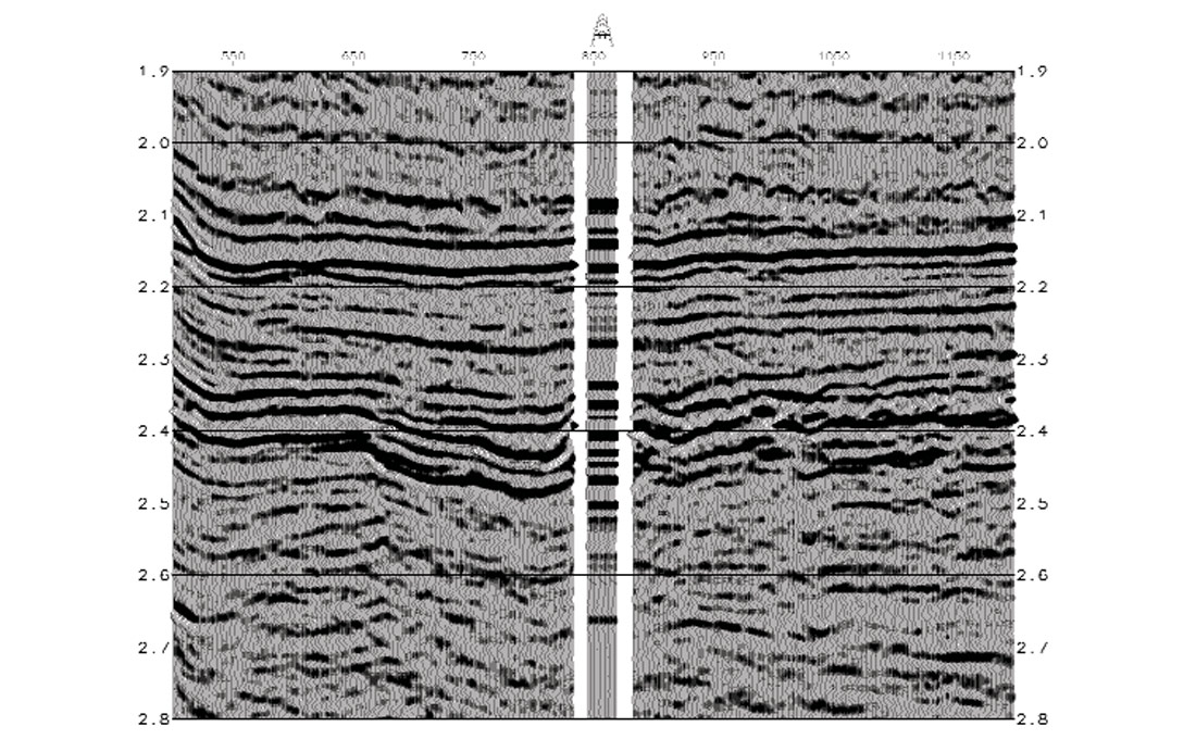
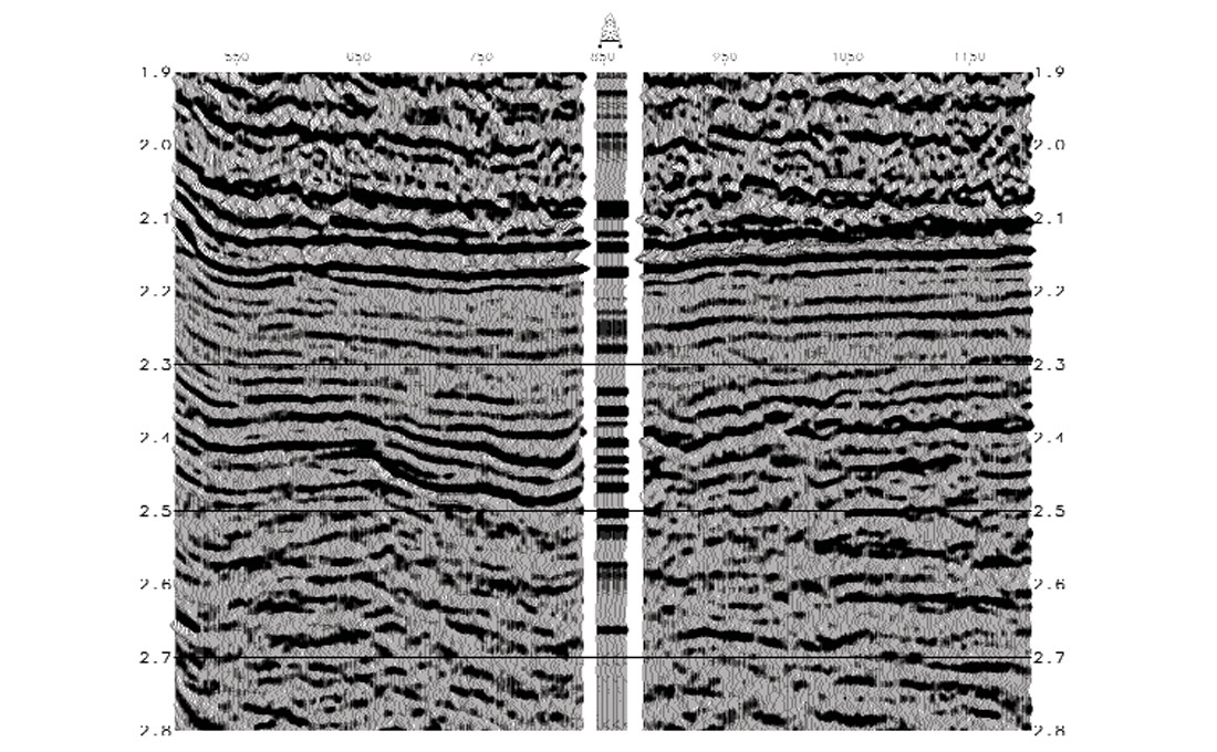
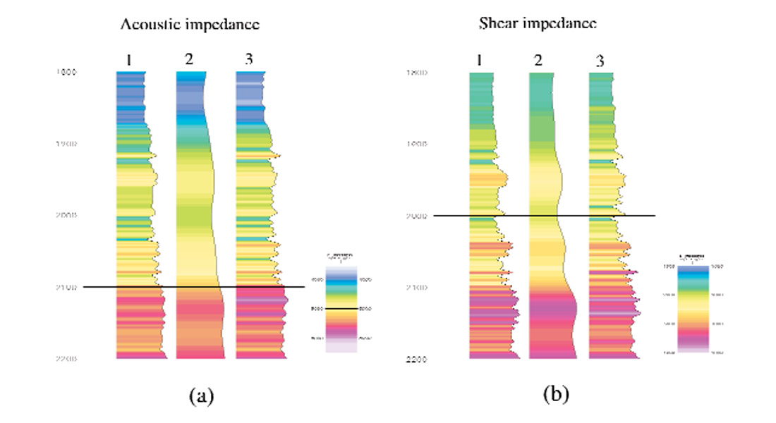
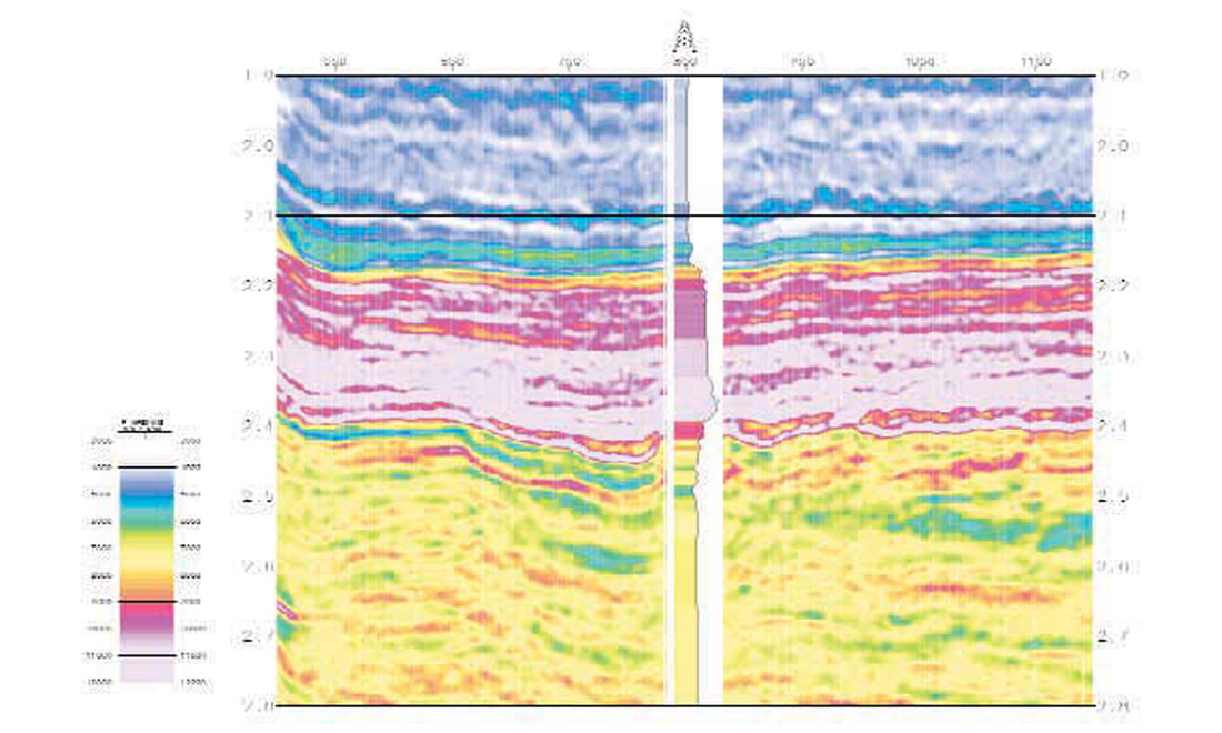
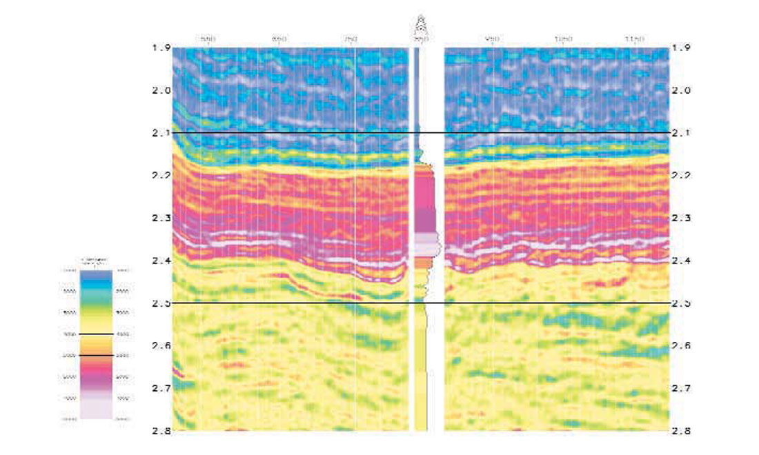
The CMP gathers and low frequency Vs/Vp ratios were input into an AVO extraction program. The output of AVO analysis are stacks of 'zero-offset P-wave' reflectivity series (Figure 7a) and 'zero-offset S-wave' reflectivity series (Figure 7b). The joint inversion algorithm takes 5 data sets as input; they are P- and S-seismic, low frequency P- and S- impedance and wavelets. It outputs both acoustic (Ip) and shear (Is) impedance traces. Figures 7a and 7b show the impedance results for a seismic inline crossing the well. It can be seen that the inverted P- and S- impedance show a very high vertical resolution and a lateral consistency. The well match is also very good. These results demonstrate the stability and robustness of the global joint inversion in estimating acoustic and shear impedance needed for reservoir characterisation.

Rock properties derived from P- and S- impedance

Acoustic and shear impedance estimated using the new global joint inversion scheme can be used to derive the conventional rock properties such as Vs/Vp, Poisson's ratio (σ) and Poisson reflectivity. Recently Goodway et al. (1997) have introduced the technique of using Lamé's constants (λ and μ) to discriminate gas sand from shales. This technique was based on the fact that λ values represent incompressibility; gas zones are zones of low incompressibility, while μ gives information about the rigidity of the rock matrix; the rock matrix will remain unaffected by the nature of the pore fluid. The λρ and μρ are directly derivable from acoustic and shear impedance by λρ = Ip²-2Is² and μρ = Is² (See Goodway et al. for derivations). Cross-plotting λρ versus μρ or λρ versus λ/μ enables fluid content and lithology to be discriminated. The crossplots using Lamé's constants have shown to be better hydrocarbon indicators than the conventional crossplots via (Vp, Vs) and (Ip, σ).

Conclusions

For reservoir characterisation, seismic reflectivity data must be inverted to rock properties. The developed joint inversion algorithm proves to be capable of producing both acoustic and shear impedance with a great efficiency and a high resolution. The use of both P- and S wave information can make a significant impact on the non-uniqueness problem in many cases of lithology and fluid discrimination.

Acknowledgements

The author thanks Paul Haskey, Adrian Pelham and Michael Burianyk of Scott Pickford Group Ltd for the stimulating discussion and valuable comments on this work. The author also thanks Techmarine International Ltd. for providing the North Sea data for the test of the joint inversion method.